Tutorial on Quantum Espresso

In this section, I would like to describe the procedures that I used to conduct first-principles simulation on the electronic structures and material properties and gain hand-on experiences of quantum espresso. The newest version of QE will be used. You can refer to my webpage for how to install the package and the libraries needed. Here I use silicon and aluminum to illustrate the simulation procedures on semiconductor and metal, respectively. You can download the structural files from ICSD or any other public domain database and build the crystal structure with xcrysden, VESTA or any crystal builder. After we have the unit cell information, the unit cell structure of a crystalline material is always relaxed and then self consistent calculation (scf) is completed. After that, we can estimate the elastic modulus of the crystals and calculate its band structure. Along this line, we will analyze the density of states to learn what atomic orbitals contribute significantly to the occupied and unoccupied bands.

Semiconductor: Silicon

A. Structural Relaxation

A structural relaxation can be done by specifying the 'calculation' flag with either 'relax' or 'vc-relax' (vc meaning variable cell). The difference between the two is that in 'vc-relax' the cell parameter itself is allowed to change, whereas in 'relax' the cell is fixed but the atoms can move within the cell. You can prepare an input file to run quantum espresso module pw.x. To save your effort, you can download a shell script "Si-vcrelax.sh" here to automate the process. Run the shell script as follows:
  $ mkdir 1a_stropt | cd 1a_stropt
  $ ./Si-vcrelax.sh

The script will produce the input file "Si.vcrelax.in" and generate the output files: Si.vcrelax.out. Find out the new lattice parameter from the output with an awk command:
  $ awk '/CELL_/{x=NR+3}(NR<=x){print}' Si.vcrelax.out
  --> CELL_PARAMETERS (alat= 10.26000000)
  -0.501241493   0.000000000   0.501241493
  -0.000000000   0.501241493   0.501241493
  -0.501241493   0.501241493   0.000000000
    CELL_PARAMETERS (alat= 10.26000000)
  -0.502599800   0.000000000   0.502599800
  +0.000000000   0.502599800   0.502599800
  -0.502599800   0.502599800   0.000000000
    CELL_PARAMETERS (alat= 10.26000000)
  -0.502599800   0.000000000   0.502599800
  +0.000000000   0.502599800   0.502599800
  -0.502599800   0.502599800   0.000000000

An original lattice vector belongs to the family (0.5 0.5 0.0), so we can compute our new lattice vector by (0.502599800/0.5) x 10.26 = 10.31335 [bohr] = 5.4558 [Angstrom].

B. SCF Run

1. Prepare an input file for silicon scf run with calculation = 'scf' and celldm(1) = 10.31335
  You can download the si.scf.in here.

2. Execute the script:
  $ mpirun -np 12 --map-by core /opt/QE540/pw.x < si.scf.in > si.scf.out
  --> (12 mpi processes, 1 threads-per mpi process, effective 12 cores)
    PWSCF : 0.32s CPU 0.37s WALL
    This run was terminated on: 22:36:17 28Aug2016

3. Check the output
  $ grep ! si-scf.out | awk '{print $5}'
  --> -15.75147877 Ry

C. Equation of State (EoS)

1. Prepare the shell script volume.sh
  $ chmod +x volume.sh

2. Calculate the total energy as a function of lattice constant
  $ ./volume.sh
  --> volume.dat

3. Equation of State (EoS) Fit with the Python script eos-fit.py
  $ chmod +x eos-fit.py
  $ ./eos-fit.py
  --> Welcome to eos-fit.py
  Filename containing energy vs volume [volume.dat]: volume.dat
  Volume or lattice spacing (vol/latt) [default=vol]: vol
  Lattice units (ang/bohr) [default=ang]: ang
  Energy units (eV/Ry/Ha) [default=eV]: eV
  Murnaghan : E0 = -15.751603 eV
  Murnaghan : B0 = 0.961747 GPa
  Murnaghan : Bp = 3.584726
  Murnaghan : V0 = 276.233865 angstrom^3
  Do you want to plot the result (yes/no) [default=yes]: yes
  Save the figure file si.eos.png

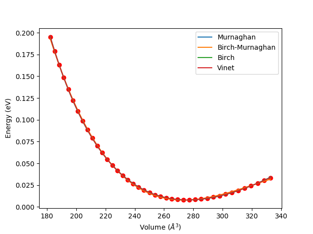
FIG.1: Equation of state (EoS) of silicon single crystal.

D. Charge Density Plot on a Specific Plane

1. Prepare a shell script run-si.scf.sh for scf calculation. Execute the code with
  $ ./run-si.scf.sh
  --> which produces si.scf.out

2. Check the result
  $ grep -e '! total energy' si.scf.out
  -->   !   total energy     =   -15.74127070 Ry

3. Postprocess charge density data on a specific plane using run-si.pp.sh script:
  $ ./run-si.pp.sh
  --> si.pp.out   si.charge   si.rho110.dat

4. Process si.rho110.dat into a figure file si.rho110.ps:
  $ /opt/QE540/plotrho.x
  --> Input file > si.rho110.dat
  r0 :   0.0000   0.0000   0.0000
  tau1 :   1.0000   1.0000   0.0000
  tau2 :   0.0000   0.0000   1.0000
  read   2 atomic positions
  output file > si.rho110.ps
  Read 56 * 40 grid
  Logarithmic scale (y/n)? > n
  Bounds:   0.003078   0.084520
  min, max, # of levels > 0.003, 0.085, 10

5. Observe the figure
  $ xdg-open si.rho110.ps

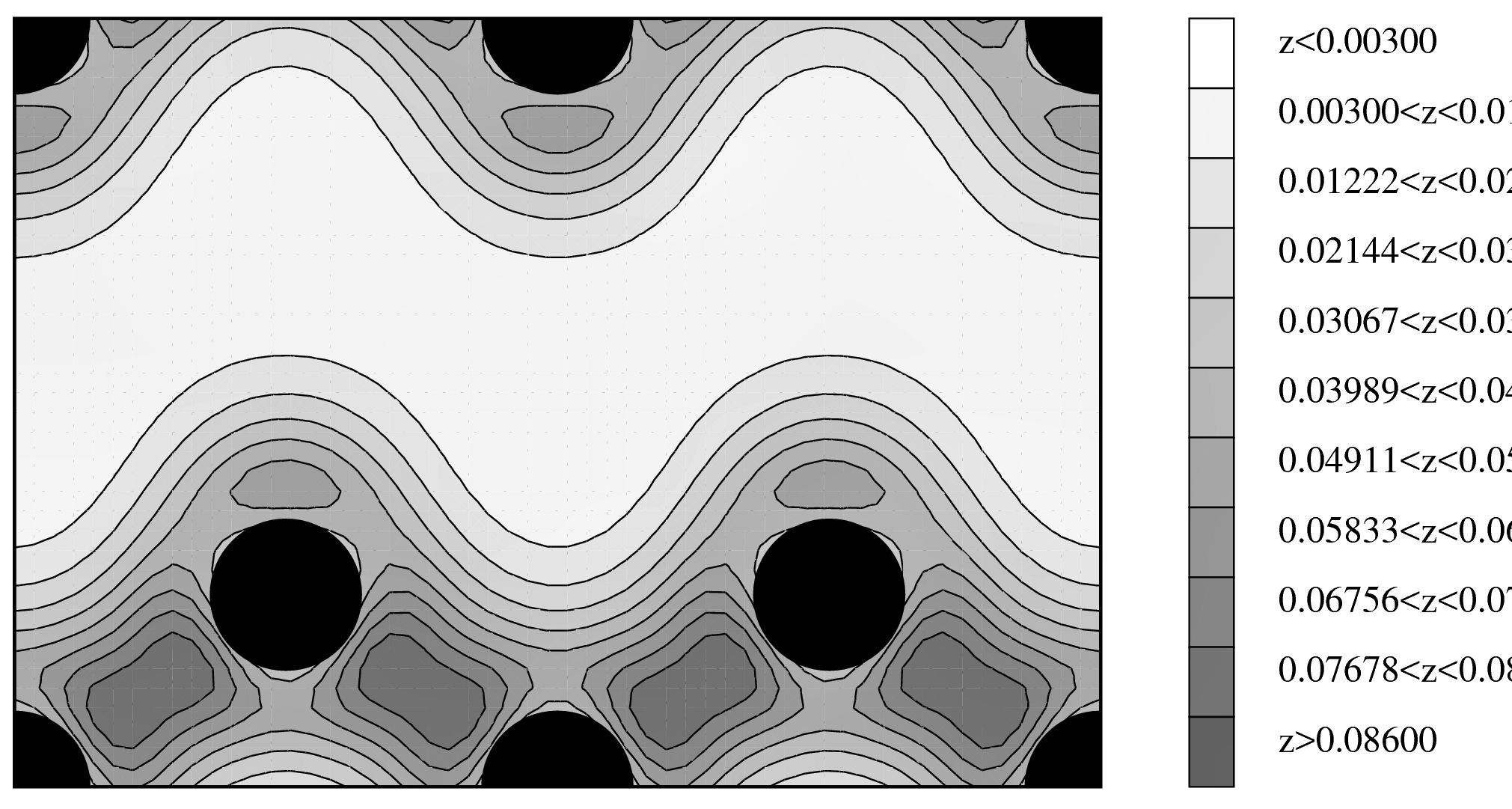
FIG.2: Charge density plot on (110) plane of silicon crystal.

E. Conduct a nscf Run for Analyzing Density of State

1. Prepare a shell script run-si.nscf.sh for nscf calculation on 6x6x6 k-mesh. Execute the code with
  $ ./run-si.nscf.sh
  --> which produces si.nscf.out

2. Check the result
  $ grep -e "End of band structure calculation" si.nscf.out -A 9
  --> End of band structure calculation
    k = -0.0833   0.0833   0.0833   ( 749 PWs)   bands (ev) :
    -5.6377   5.2285   5.9326   5.9326   8.6761   8.8475   8.8475   10.0331
    13.5285   13.5285   14.4008   16.9798
  occupation numbers
    1.0000   1.0000   1.0000   1.0000   0.0000   0.0000   0.0000   0.0000
    0.0000   0.0000   0.0000   0.0000
  highest occupied level (ev) : 5.9326 eV

3. Producing DOS plot with run-si.dos.sh and execute the code.
  $ ./run-si.dos.sh
  --> which produces si.dos.out   si.dos [E(eV) dos(E) Int dos(E)]
  Prepare the dos figure with dos.gnu
  $ gnuplot dos.gnu
 --> si.dos.ps
  Observe the plot with
  $ xdg-open si.dos.ps

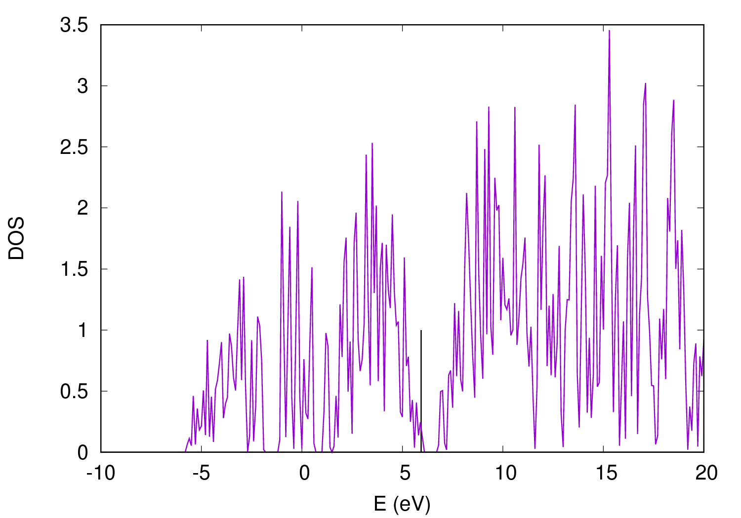
FIG.3: Density of state (DoS) plot of silicon crystal. The vertical line at 5.93 eV marks the highest occupied level.

4. Producing Partial DoS plot with run-si.pdos.sh and execute the code.
  $ ./run-si.pdos.sh
  --> which produces si.pdos.out   si.pdos_tot
  si.pdos_atm#1(Si)_wfc#1(s) si.pdos_atm#1(Si)_wfc#2(p) si.pdos_atm#2(Si)_wfc#1(s) si.pdos_atm#2(Si)_wfc#2(p)

  Prepare the pdos figure with pdos.gnu
  $ gnuplot pdos.gnu
 --> si.pdos.ps
  Observe the plot with
  $ xdg-open si.pdos.ps

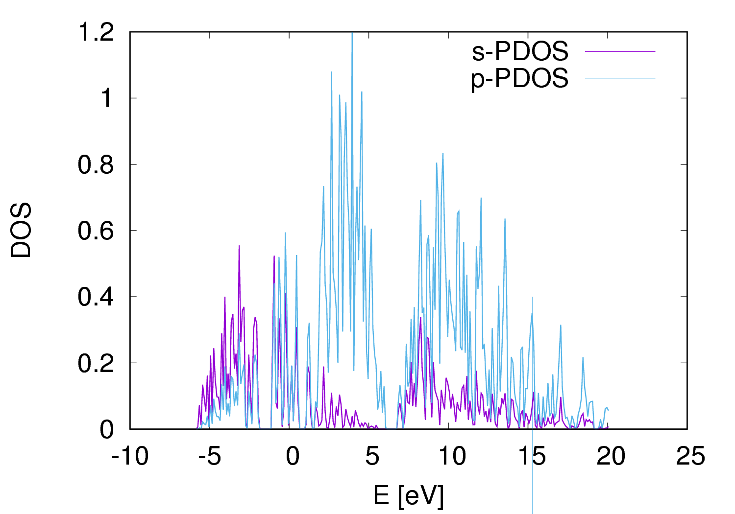
FIG.4: Partial density of state (pDoS) plot of silicon crystal. As seen the near band edge states are dominated by Si-p orbitals.

F. Band Structure Calculation

1. Prepare an input file si-bands.in for nscf calculation along the high symmetry paths in the first Brillouin zone. Execute the calculation with
  $ mpirun -np 12 --bind-to core /opt/QE540/pw.x si-bands.out

2. Collect the band results for plotting using the code bands.x, which reads data file(s), extracts eigenvalues, regroups them into bands. The output is written to a file that can be directly read and converted to plottable format. A shell script plot_bandstr.sh is prepared to automate this plotting process.
  $ ./plot_bandstr.sh
  --> gnuplot_bandstr.eps gnuplot_dos.eps

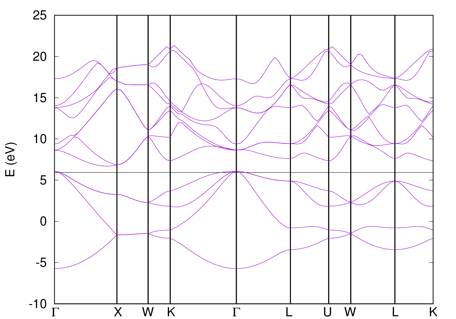
FIG.5: Bandstructure of silicon crystal.

Metallic Crystal: Aluminum

A. SCF Run for visualizing charge density distribution

1. Prepare a shell script run-al.scf.sh for scf calculation. Execute the code with
  $ ./run-al.scf.sh
  --> which produces al.scf.out

2. Check the result
  $ grep -e '! total energy' al.scf.out
  -->   !   total energy     =   -4.18794320 Ry

3. Postprocess charge density data on a specific plane using run-al.pp.sh script:
  $ ./run-al.pp.sh
  --> al.pp.out   al.charge   al.rho110.dat

4. Process al.rho110.dat into a figure file al.rho110.ps:
  $ /opt/QE540/plotrho.x
  --> Input file > al.rho110.dat
  r0 :   0.0000   0.0000   0.0000
  tau1 :   1.0000   1.0000   0.0000
  tau2 :   0.0000   0.0000   1.0000
  read   1 atomic positions
  output file > al.rho110.ps
  Read 56 * 40 grid
  Logarithmic scale (y/n)? > n
  Bounds:   0.000135   0.032490
  min, max, # of levels > 0.0001, 0.033, 10

5. Observe the figure
  $ xdg-open al.rho110.ps

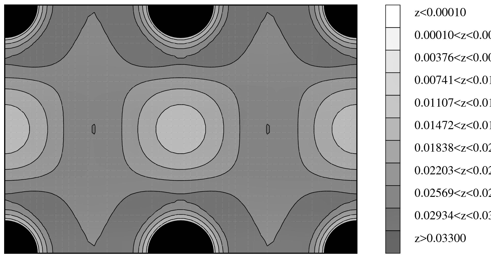
FIG.6: Charge density plot on (110) plane of aluminum crystal.

B. Conduct a nscf Run for Analyzing Density of State

1. Prepare a shell script run-al.nscf.sh for nscf calculation on 8x8x8 k-mesh. Execute the code with
  $ ./run-al.nscf.sh
  --> which produces al.nscf.out

2. Check the result
  $ grep -e "End of band structure calculation" al.nscf.out -A 5
  --> End of band structure calculation
    k = -0.0625   0.0625   0.0625   ( 169 PWs)   bands (ev) :
    -3.4125   20.1308   20.1308   20.1308   21.0611   21.0611   21.0611   23.9319

3. Producing DOS plot with run-al.dos.sh and execute the code.
  $ ./run-al.dos.sh
  --> which produces al.dos.out   al.dos [E(eV) dos(E) Int dos(E)]
  Prepare the dos figure with dos.gnu
  $ gnuplot dos.gnu
 --> al.dos.ps
  Observe the plot with
  $ xdg-open al.dos.ps

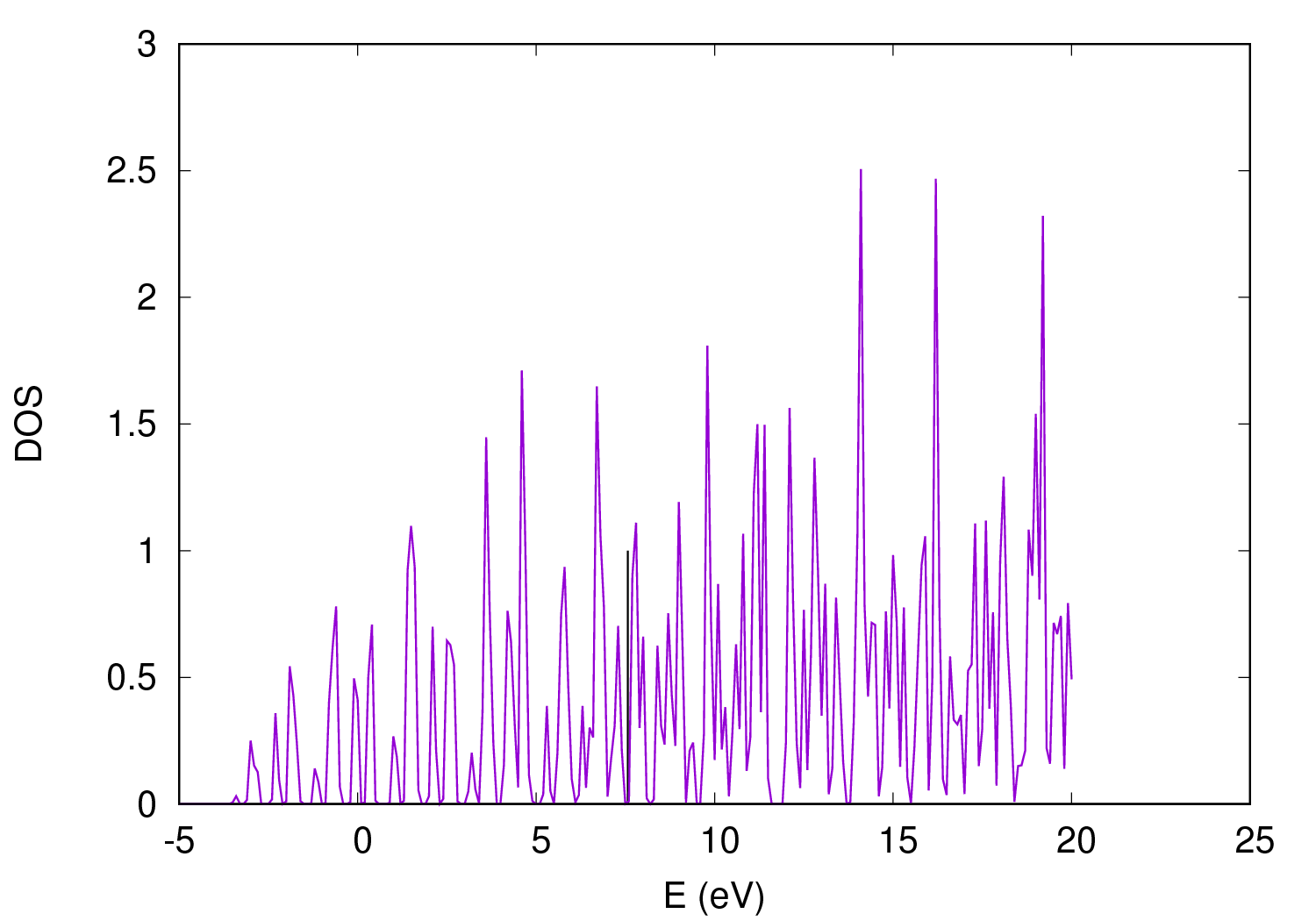
FIG.7: Plot of density of state of Al crystal.

4. Producing Partial DoS plot with run-al.pdos.sh and execute the code.
  $ ./run-al.pdos.sh
  --> which produces al.pdos.out   al.pdos_tot
  al.pdos_atm#1(Al)_wfc#1(s) al.pdos_atm#1(Al)_wfc#2(p) al.pdos_atm#2(Al)_wfc#1(s) al.pdos_atm#2(Al)_wfc#2(p)

  Prepare the pdos figure with pdos.gnu
  $ gnuplot pdos.gnu
 --> al.pdos.ps
  Observe the plot with
  $ xdg-open al.pdos.ps

C. Band Structure Calculation

1. Prepare an input file al-bands.in for nscf calculation along the high symmetry paths in the first Brillouin zone. Execute the calculation with
  $ mpirun -np 12 --bind-to core /opt/QE540/pw.x si-bands.out

2. Collect the band results for plotting using the code bands.x, which reads data file(s), extracts eigenvalues, regroups them into bands. The output is written to a file that can be directly read and converted to plottable format. A shell script plot_bandstr.sh is prepared to automate this plotting process.
  $ ./plot_bandstr.sh
  --> gnuplot_bandstr.eps gnuplot_dos.eps

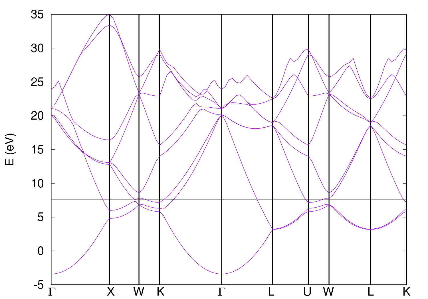
FIG.8: Bandstructure of Al.

Structural relaxation on Al(001) surface

This example demonstrates how to prepare a model for studying surface adsorption.

A. SCF without Structural Relaxation
1. I will perform an scf calculation of Al(001) slab without structural relaxation. First, prepare an input file al001-scf.in for the scf run. Selecting ibrav = 6 to indicate a tetragonal structure with celldm(3)=c/a for v1 = a(1, 0, 0), v2 = a(0, 1, 0), v3 = a(0, 0, c/a).
  $ mkdir 1d_Al001stropt | cd 1d_Al001
  $ mpirun -np 12 --map-by core /opt/QE540/pw.x < al001-scf.in > al001-scf.out

2. Find out the total energy from the output with a grep command:
  $ grep "! total" al001-scf.out
  --> !   total energy = -20.88053599 Ry

3. Analyse the forces (Note: tprnfor = .true.)
  $ cat al001-scf.out | grep -e "Forces acting on atoms (Ry/au)" -A 8
  -> Forces acting on atoms (Ry/au):
    atom 1   type 1   force = 0.00000000   0.00000001   -0.01593286
    atom 2   type 1   force =-0.00000000   -0.00000000   0.00618552
    atom 3   type 1   force = 0.00000002   -0.00000000   0.00000037
    atom 4   type 1   force =-0.00000002   -0.00000001   -0.00618583
    atom 5   type 1   force = -0.00000000   0.00000000   0.01593279

    Total force = 0.024171   Total SCF correction = 0.000048

    Are the atomic forces pointing outward or inward? Outward.

B. SCF with Structural Relaxation

1. Structural relaxation of Al(001) slab can be done by specifying the 'calculation' flag with 'relax', which allows atoms to relax in the supercell. Modify the input file to perform a structural relaxation with the BFGS method and save the new input as al001-BFGS.in
  calculation = "relax": relax atom positions whereas keep cell dimensions unchange
  bfgs_ndim=3: 3 old forces and displacements vectors were used in the PULAY mixing of the residual vectors.
  upscale : conv_thr/upscale, which is the max reduction factor for conv_thr during structural optimization.

2. Execute the script:
  $ mpirun -np 12 --map-by core /opt/QE540/pw.x al001-BFGS.out

3. Analyse the forces:
  $ cat al001-BFGS.out | grep -e "Forces acting on atoms (Ry/au)" -A 8
  -> Forces acting on atoms (Ry/au):
    atom 1   type 1   force = 0.00000016   -0.00000012   -0.00018726
    atom 2   type 1   force = -0.00000010   -0.00000004   0.00036627
    atom 3   type 1   force = -0.00000027   0.00000041   -0.00020878
    atom 4   type 1   force = 0.00000024   -0.00000032   -0.01340351
    atom 5   type 1   force = -0.00000004   0.00000007   0.01343329

    (relaxed) Total force = 0.000461   Total SCF correction = 0.000027

    (wo relax) Total force = 0.024171   Total SCF correction = 0.000048

Oxygen Adsorbed on Al(100)

A longstanding problem on ab initio calculation is to visualize the charge redistribution and transfer caused by an adsorbate on a metal surface. In this example, I will show how to do it.

A. O-Al(100) System

1. For the system of oxygen atom adsorbed on Al(100) surface, we need to run the scf calculation of oxygen atom, Al(100) slab, and O-Al(100). A shell script run-Al-O-OAl.sh was prepared to automate the calculations:
  $ ./run-Al-O-OAl.sh
 --> O.scf.out, Al.scf.out, OAl.scf.out

2. After these scf runs, we can then extract the charge density for the O/Al(001) system (OAl.scf.out), the O alone (O.scf.out), the Al alone (Al.scf.out) and get the difference rho(O/Al)-rho(O)-rho(Al) with a shell script run-OAl.chdiff.sh
  $ ./run-OAl.chdiff.sh

3. Visualize the result with
  $ xcrysden --xsf OAl.chdensDIFF.xsf

  In Xcrysden: Choose
  Tools-> DataGrid
  Select: Display Isosurface
  Isovalue: 0.002 and
  Select: render +/- isovalue
  Transparency of isosurface: on
  Adjust Transparency:
  Specify source blending type: GL_ONE_MINUS_DST_ALPHA
  Specify destination blending type: GL_ONE_MINUS_SRC_COLOR

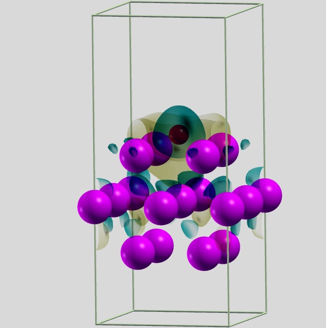
FIG.1: Plot of charge difference of O-Al(100).

ESM Model for Electrochemistry

Electrochemistry is an extremely important topics in energy generation and storage. In this section, a case study is presented to show the simulation steps with the Effective Screening Medium (ESM) model, which can be used to yield the total energy, charge density, force, and potential of a polarized or charged medium. ESM screens the electronic charge of a polarized/charged medium along one (perpendicular to the interfaces) direction by introducing a classical charge model and a local relative permittivity into the first-principles calculation framework. This permits calculations using open boundary conditions (OBC). The method was described in detail in M. Otani and O. Sugino, "First-principles calculations of charged surfaces and interfaces: A plane-wave nonrepeated slab approach," PRB 73, 115407 (2006).

In addition to 'pbc' (ordinary periodic boundary conditions with ESM disabled), the code allows three different sets of boundary conditions perpendicular to the polarized medium:
  I) 'bc1' : Immerse the medium between two semi-infinite vacuum regions;
  II) 'bc2' : Immerse the medium between two semi-infinite metallic electrodes, with optional fixed field applied between them;
  III) 'bc3' : Immerse the medium between one semi-infinite vacuum region and one semi-infinite metallic electrode.

This case study is organized as follows:
  I. esm_bc = 'bc1':
    A). Make a self-consistent calculation for H2O with esm_bc = 'pbc' (ESM off)
    (input=H2O.noesm.in, output=H2O.noesm.out). Using 'pbc' causes the code to print out the density and potential (hartree + local) along z, even though ESM is disabled. Note that the molecule has a z-oriented dipole.
    B) Make a self-consistent calculation for H2O with esm_bc = 'bc1'
    (input=H2O.bc1.in, output=H2O.bc1.out). This simulates the water molecule in an infinite vacuum along the z-direction, preventing dipole-dipole interaction between periodic images.

  II. esm_bc = 'bc2':
    A) Make a self-consistent calculation for Al(111) with esm_bc = 'bc2', without an applied field
    (input=Al111.bc2.in, output=Al111.bc2.out). This simulates the slab sandwiched between two uncharged semi-infinite metal electrodes.
    B) Make a self-consistent calculation for Al(111) with esm_bc = 'bc2', this time with an applied field
    (input=Al111.bc2_efield.in, output=Al111.bc2_efield.out). The slab polarizes in response.

  III. esm_bc = 'bc3':
    A) Make a self-consistent calculation for Al(111) with esm_bc = 'bc3' to simulate a semi-infinite system in contact with vacuum
    (input=Al111.bc3.in, output=Al111.bc3.out).
    B) Make a self-consistent calculation for Al(111) with esm_bc = 'bc3' to simulate a semi-infinite system in contact with vacuum with a weakly negative (-0.005e) overall charge
    (input=Al111.bc3_m005.in, output=Al111.bc3_m005.out). Note that the charge migrates to the surface/vacuum interface.
    C) Repeat III.2 but with a weakly positive (+0.005e) overall charge
    (input=Al111.bc3_p005.in, output=Al111.bc3_p005.out).

Simulation Steps

1. A shell script runESM.sh can be downloaded here to facilitate the calculation:
  $ ./runESM.sh

2. Analyze the results:
  $ cd ./results

  I.A) H2O in cell with pbc
  $ grep -e "the Fermi energy" H2O.noesm.out
  --> the Fermi energy is -4.0771 ev
  $ grep -e "!   total energy" H2O.noesm.out
  --> !   total energy     = -34.25356994 Ry
  $ grep -e "negative rho" H2O.noesm.out
  --> negative rho (up, down): 2.901E-04 0.000E+00

  I.B) H2O in an infinite vacuum along the z-direction
  $ grep -e "the Fermi energy" H2O.bc1.out
  --> the Fermi energy is -4.1845 eV
  $ grep -e "!   total energy" H2O.bc1.out
  --> !   total energy     = -34.25323086 Ry
  $ grep -e "negative rho" H2O.bc1.out
  --> negative rho (up, down): 2.900E-04 0.000E+00

  II.A) Al(111) slab sandwiched between two uncharged semi-infinite metal electrodes
  $ grep -e "the Fermi energy" Al111.bc2.out
  --> the Fermi energy is -4.0072 eV
  $ grep -e "!   total energy" Al111.bc2.out
  --> !   total energy     = -28.92859648 Ry

  II.B) Al(111) slab sandwiched between two uncharged semi-infinite metal electrodes with an e-field along z
  $ grep -e "the Fermi energy" Al111.bc2_efield.out
  --> the Fermi energy is   -3.0085 ev (which is shifted upward from -4.0072 eV)
  $ grep -e "!   total energy" Al111.bc2_efield.out
  --> !   total energy     = -27.38458670 Ry

  III.A) A semi-infinite Al(111) system in contact with vacuum
  $ grep -e "the Fermi energy" Al111.bc3.out
  --> the Fermi energy is -4.0069 eV
  $ grep -e "!   total energy" Al111.bc3.out
  --> !   total energy     = -28.92859747 Ry

  III.B) A semi-infinite Al(111) system in contact with vacuum with -0.005e charge
  $ grep -e "the Fermi energy" Al111.bc3_m005.out
  --> the Fermi energy is -2.5441 ev (which is shifted upward from -4.0069 eV)
  $ grep -e "!   total energy" Al111.bc3_m005.out
  --> !   total energy     = -28.92980080 Ry (no significant change!)

  III.C) A semi-infinite Al(111) system in contact with vacuum with +0.005e charge
  $ grep -e "the Fermi energy" Al111.bc3_p005.out
  --> the Fermi energy is -5.4731 ev (which is shifted downward from -4.0069 eV)
  $ grep -e "!   total energy" Al111.bc3_p005.out
  --> !   total energy     = -28.92718160 Ry (does not change significantly!)

Ferromagnetism

In this section, I will describe the simulation procedures for ferromagnetic crystal. BCC iron was chosen for this case study. First, we will compute total energy and magnetization versus the lattice parameter with reveal the most stable dimension of the unit cell. By using this unit cell dimension, we will compute the spin-polarized band structure of Fe.bccFM (pw.x + bands.x). After that, we compute the spin-polarized density of states of Fe.bccFM(pw.x + projwfc.x). Finally, fixed spin moment (fsm) calculation was performed at various lattice parameters of fcc Fe to display the difference with that of bcc Fe.

A. Total Energy and Magnetization of BCC Iron Crystal versus Lattice Constant

To save your effort, you can download a shell script "pw.alat.sh" here to automate the simulation work. This script can run pw.x for several lattice parameters (the output files are stored in a single file by using the double redirection >>). A simple bash command (grep+awk) is searching for the total energy and total magnetization of the system. Run the shell script as follows:
  $ ./pw.alat.sh
The script will produce two output files that are stored in ./results.alat/Fe.bccFM.etot_vs_lattice and ./results.alat/Fe.bccFM.mag_vs_lattice. To visualize the figures, prepare the gnuplot script etot.gnu: and execute the following command:
  $ gnuplot etot.gnu

Yo visualize the plots, use
  $ xdg-open etot.alat.eps
  $ xdg-open mag.alat.eps

 

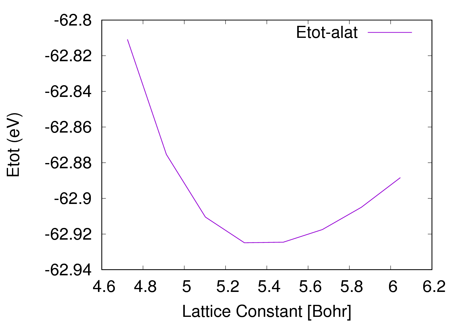
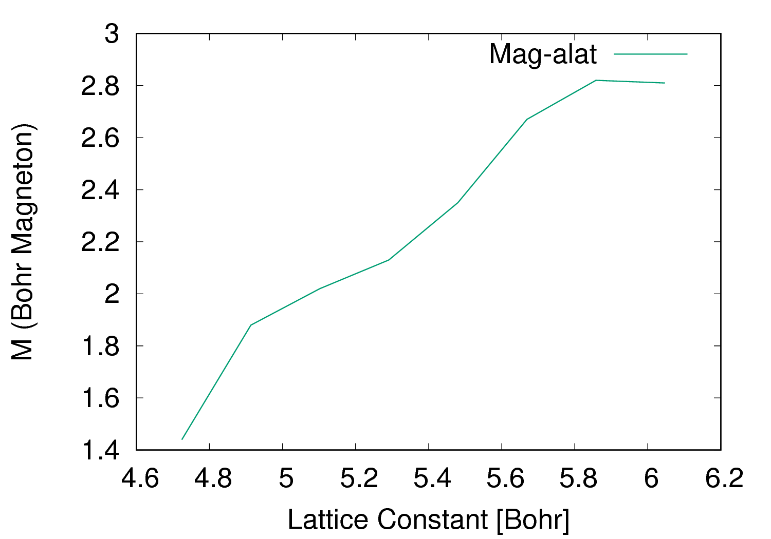
FIG.1: Total energy and magnetization of ferromagnetic bcc iron crystal plotted as a function of lattice constant (Bohr).

B. Compute the spin-polarized band structure of Fe.bccFM

The band structure is performed in three steps:
  a) First perform an scf pw.x calculation and then
  b) Perform an nscf calculation for a given K-path in the Brillouin zone. There are differents ways of entering the K-Path. Either explicitely or by the option K_POINTS (tpiba_b) that allows you to draw lines between extremal points. This is the option that we have used. Finally,
  c) Use bands.x to post-process the result and generate the band-structure (kx,ky,kz, E(kx,ky,kz)) for up and down spin polarized bands. Plot the band structure with plotband.x.

All the steps are automated with the shell script pw.bands.sh, which can be downloaded here. Execute this script:
  $ ./pw.bands.sh
and then
  $ cd ./results.band

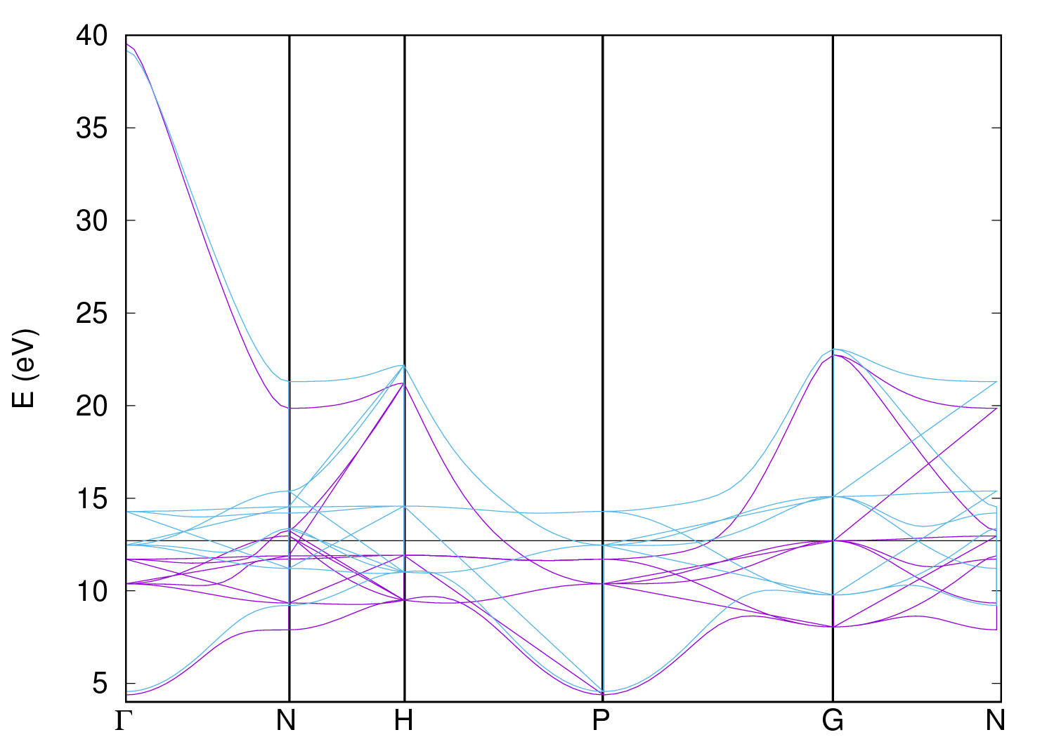
FIG.2: Spin polarized Bandstructure of Fe.bccFM.

C. Spin Polarized Density of States of Fe.bccFM

The DOS can be calculated in three steps:
  a) First conduct scf pw.x calculation and then
  b) Perform nscf calculation with a larger number of K-point to have a smoother DOS(E) curve. Finally,
  c) projwfx.x is used to post-process and project the Kohn Sham wave functions onto the pseudo-atomic wave functions with a Lowdin procedure.

Compare the atomic-projected magnetization (output of projwfc.x) and the magnetization integrated in a sphere (output of pw.x).
Apart from the general output, a large number of files containing the projected DOS come out of projwfc.x (number of atoms x number of orbitals per atom).
Since there is only one atom in the unit-cell we get only 3 files for s,p and d orbitals. The format of "Fe.bccFM.pdos.pdos_tot" is basically of the form:
E   DOSup(E)   DOSdw(E)   PDOSup(E)   PDOSdw(E)

All the steps are automated with the shell script pw.dos.sh, which can be downloaded here. Execute this script:
  $ ./pw.dos.sh
The dos and pdos plots are stored in ./results.dos folder
  $ cd ./results.dos

 

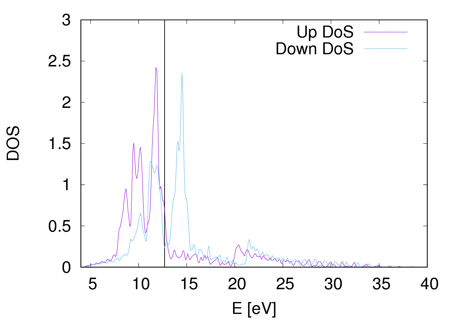
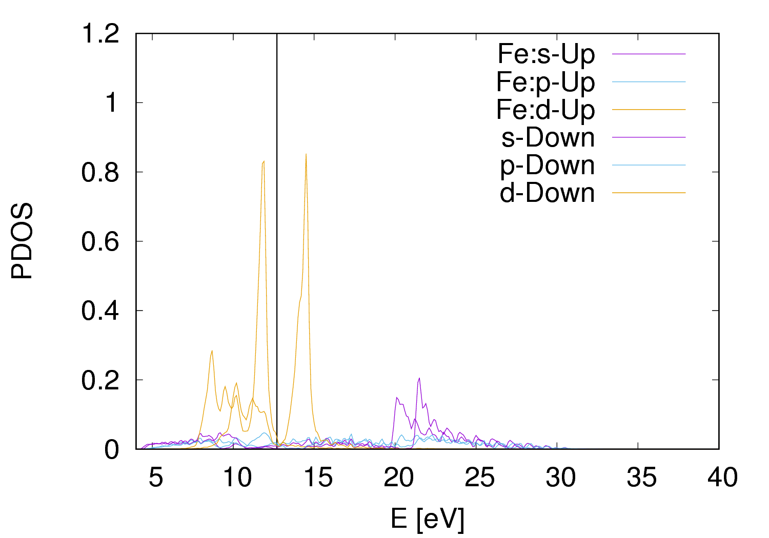
FIG.3: Plots of density of state (Left) and partial density of states (Right) of Fe.bccFM crystal. The vertical line at 12.5 eV marks the position of the Fermi level.

D. Fixed spin moment (fsm) calculation at various lattice parameters of Fe.fcc.FM

The structure considered is Fe.fcc, which has a more complex magetic behavior. In particular, two magnetic solution (Low spin and High Spin) are coexisting in a range of lattice parameters.
Execute pw.fsm.sh to run a series of pw.x scf calculations with the option of tot_magnetization = M that fixes the total magnetization to a given value. The bash script is then extracting the curve E(M) that is stored in Fe.fccFM.etot_vs_mag
  $ ./pw.fsm.sh
and then
  $ cd ./results.fsm
Plot E(M) at various lattice parameters. What do you notice for lattice parameters around 3.55 Angstroms?

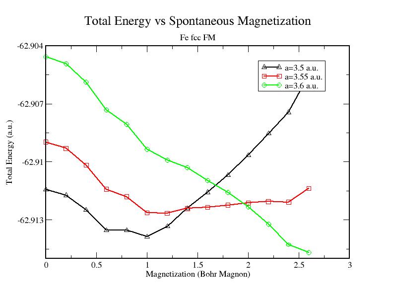
FIG.4: Total energy vs spontaneous magnetization of Fe.fccFM crystal.

Ferroelectricity: Berry Phase for Electric Polarization

In this study, we will learn how to use Berry phase formalism of electric polarization to calculate the electric and ionic polarizations for symmetric (A) and asymetric (B) BaTiO3 crystals. To probe into this issue deeply, the effective Born charge generated by displacing the central Ti atom from its symmetric lattice position (C) is also calculated to reveal the origin of the electric polarizations.

A. Calculate Polarization via Berry Phase for Symmetric Tetragonal BaTiO3

1. Do a pw scf calculation of total energy on the equilibrium structure with well converged k-mesh and ecutwfc. Prepare the input file "sy.scf.in" with ibrav= 6, K_POINTS=5 5 5.
2. Execute the command:
  $ mpirun -np 12 --map-by core /opt/QE540/pw.x < sy.scf.in > sy.scf.out
3. Check final total energy
  $ grep -e 'highest occupied level' sy.scf.out -A 4
  --> highest occupied level (ev):   10.3313

  !   total energy     = -303.29721697 Ry
  Harris-Foulkes estimate = -303.29721697 Ry
  estimated scf accuracy < 1.2E-09 Ry

4. Run nscf with input file "sy.bscf.in" to evaluate the Berry phase along selected k-point strings.
  $ nano sy.bscf.in
  Note: ibrav= 6, K_POINTS=5 5 10 in the &control field:
  lberry=.true. (for doing nscf via Berry phase)
  gdir = 3 (direction of the k-point strings in reciprocal space. Allowed values: 1, 2, 3 where 1= first, 2= second, 3=third reciprocal lattice vector).
  nppstr= 10 (Number of k-points in the string along gdir).

  $ mpirun -np 12 --map-by core /opt/QE540/pw.x < sy.bscf.in > sy.bscf.out

5. Check total polarization = ionic part + electronic part
  $ grep -e "highest occupied level" sy.bscf.out
  --> highest occupied level (ev): 10.3313

  $ grep -e "IONIC PHASE" sy.bscf.out
  --> IONIC PHASE:   0.00000 (mod 2)

  $ grep -e "ELECTRONIC PHASE" sy.bscf.out
  --> ELECTRONIC PHASE:   0.00000 (mod 2)

  $ grep -e "SUMMARY OF PHASES" sy.bscf.out -A 5
  --> SUMMARY OF PHASES
    ~~~~~~~~~~~~~~~~~
    Ionic Phase:   0.00000 (mod 2)
    Electronic Phase:   0.00000 (mod 2)
    TOTAL PHASE:   0.00000 (mod 2)

B. Electric and Ionic Polarizations of BaTiO3 with Asymmetric Lattice Structure

Optimize the structure of tetragonal BaTiO3 with displaced Ti atom, and then calculate the polarization via Berry phase.

1. Do a pw relax calculation. Prepare the input file "relax.in" (calculation = 'relax', tprnfor = .true., ibrav= 6, with a displaced Ti atom along z).
2. Execute the command:
  $ mpirun -np 12 --map-by core /opt/QE540/pw.x < relax.in > relax.out
3. Check the result
  $ grep -e '!   total energy' relax.out
  --> !   total energy   =   -303.29995134 Ry

  $ grep -e 'ATOMIC_POSITIONS' relax.out -A 6
  --> ATOMIC_POSITIONS (crystal)
  Ba  0.000000000   0.000000000   0.020474751
  Ti   0.500000000   0.500000000   0.530412725
  O   0.500000000   0.500000000   -0.015431644
  O   0.500000000   0.000000000   0.492272084
  O   0.000000000   0.500000000   0.492272084

4. Subtitute the above co-ordinates to asy.scf.in and asy.bscf.in files
  $ nano asy.scf.in
  Paste the ionic coordinates into asy.scf.in

  Execute the command:
  $ mpirun -np 12 --map-by core /opt/QE540/pw.x < asy.scf.in > asy.scf.out

5. Check final total energy
  $ grep -e 'highest occupied level' asy.scf.out -A 4
  --> highest occupied level (eV): 10.3519

  !   total energy   =   -303.30014009 Ry
  Harris-Foulkes estimate   =   -303.30014009 Ry
  estimated scf accuracy   <   2.7E-09 Ry

6. Run nscf with input file "asy.bscf.in" to evaluate the Berry phase along k-point strings (gdir= 3 and nppstr=10).
  $ mpirun -np 12 --map-by core /opt/QE540/pw.x < asy.bscf.in > asy.bscf.out

7. Check total polarization = ionic part + electronic part
  $ grep -e "highest occupied level" asy.bscf.out
  --> highest occupied level (eV):   10.4689

  $ grep -e "IONIC PHASE" asy.bscf.out
  --> IONIC PHASE:   0.38438 (mod 2)

  $ grep -e "ELECTRONIC PHASE" asy.bscf.out
  --> ELECTRONIC PHASE:   -0.01728 (mod 2)

  $ grep -e "SUMMARY OF PHASES" asy.bscf.out -A 5
  --> SUMMARY OF PHASES
    ~~~~~~~~~~~~~~~~~
    Ionic Phase:   0.38438 (mod 2)
    Electronic Phase:   -0.01728 (mod 2)
    TOTAL PHASE:   0.36710 (mod 2)

  $ grep -e "VALUES OF POLARIZATION" asy.bscf.out -A 15
  -->   VALUES OF POLARIZATION
      ~~~~~~~~~~~~~~~~~~~~~~
  The calculation of phases done along the direction of vector 3 of the reciprocal lattice gives the following contribution to the polarization vector (in different units, and being Omega the volume of the unit cell):
  P =   2.8070331 (mod 15.2930243)   (e/Omega).bohr
  P =   0.0065777 (mod 0.0358362)   e/bohr^2
  P =   0.3760597 (mod 2.0488144)   C/m^2

  The polarization direction is:   ( 0.00000,  0.00000,  1.00000)

8. Spontaneous polarization of tetragonal BaTiO3
  P(asymmetric phase)-P(symmetric phase)
  = 37 uC/cm^2 - 0 uC/cm^2
  = 37 uC/cm^2

C. Effective Born Charge Generated by Displaced Ti Atom in a Cubic BaTiO3

1. Run nscf calculation with input file scf.in (ibrav= 1 with the Ti atom displaced by 0.01a along +z direction)
2. Execute the command:
  $ mpirun -np 12 --map-by core /opt/QE540/pw.x < scf.in > scf.out
3. Check final total energy
  $ grep -e 'highest occupied level' scf.out -A 4
  --> highest occupied level (eV):   14.5982

  !   total energy     =   -303.12655109 Ry
  Harris-Foulkes estimate   =   -303.12655110 Ry
  estimated scf accuracy   <   9.4E-09 Ry

2. Run a berry phase calculation along gdir=3 with input file "bscf.in".
  $ mpirun -np 12 --map-by core /opt/QE540/pw.x < bscf.in > bscf.out
3. Check the result
  $ grep -e "unit-cell volume" bscf.out
  -->   unit-cell volume   =   333.5763 (a.u.)^3

  $ grep -e "VALUES OF POLARIZATION" bscf.out -A 15
  -->   VALUES OF POLARIZATION
      ~~~~~~~~~~~~~~~~~~~~~~
  The calculation of phases done along the direction of vector 3 of the reciprocal lattice gives the following contribution to the polarization vector (in different units, and being Omega the volume of the unit cell):
  P =   0.4991262 (mod 13.8705940)   (e/Omega).bohr
  P =   0.0014963 (mod 0.0415815)   e/bohr^2
  P =   0.0855454 (mod 2.3772844)   C/m^2

  The polarization direction is:   ( 0.00000,  0.00000,  1.00000)

4. Calculate the Born Effective charge
  1 a.u. = 0.53 A = 0.53E-8 cm
  Z* = VxdP/dr = 333.6 x 8.6 [uC/cm^2] / 0.01 au = 8.1E-12 uC = 50 e

Phonon Dynamics and Thermal Conductivity of Lattice

.