|
|
|
The Laboratory of Optical Studies for Advanced Materials (LOSAM) endeavors to develop and characterize frontier materials with novel optical techniques. To pursue the goal, the laboratory is equipped with (1) high-power femtosecond laser facility, (2) widely tunable picosecond coherent light sources; and (3) Yb-doped fiber laser pumped femtosecond laser with pulse shaping apparatus, etc. To decipher the correlation of material properties with their structures and dynamics, we have developed several advanced spectroscopies and microscopies, which include infrared-visible sum-frequency vibrational spectroscopy (SFVS), 2D coherent spectroscopy (2D CS), scanning near field optical microscopy (SNOM), single-molecular tracking (SMT) and imaging (SMI) apparatus. |
Two Dimensional Coherent SpectroscopyOptical scientists have employed phase space tomography (PST) to retrieve correlation functions of light fields by measuring the intensity under spatial propagation. Similarly, physicists are endeavoring to develop quantum state tomography (QST) to recover the density matrix of a conservative quantum system under time evolution. 2D CS can be used to probe a quantum system by allowing the system to interact with a sequence of femtosecond and phase stable laser pulses. In the simplest version, a coherent femtosecond optical pulse is split into four parts. Three of the four beams are focused into the sample in a boxcar phase matching geometry. 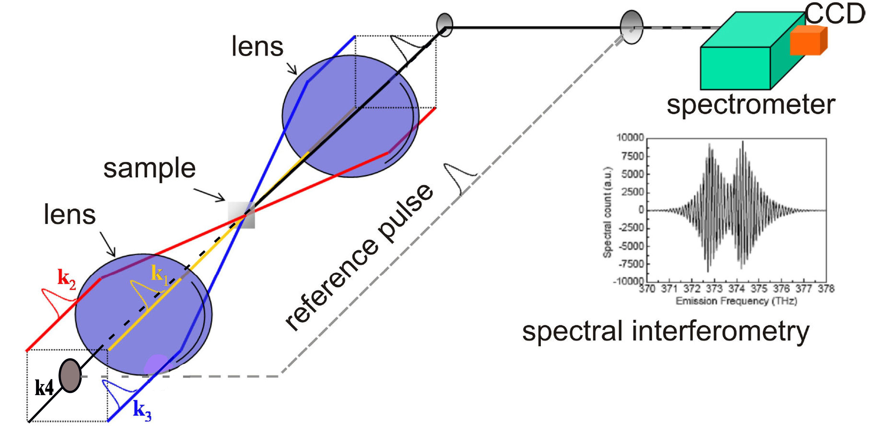
FIG. 1: Optical Setup Schematic of 2D Coherent Spectroscopy. The local oscillator pulse can be input along the echo direction (k4) or be switched out with a mirror to along a separate delay arm. An initial state is prepared by exciting the system with the first two pulses (k1 and k2) arriving at times t1 and t2, which define the coherence time interval \(t = {t_1} - {t_2}\). The time interval between the second and third pulses, called the waiting time \(T = {t_3} - {t_2}\). Varying the delay time T allows insight into the dissipative populations dynamics within the optical excitation manifold. Finally at the instant of t3, we probe the resulting density matrix with quantum state tomography (QST), which can be implemented by using the third pulse to selectively generate new dipole-active coherences. After the echo time \(\tau = {t_4} - {t_3}\) has elapsed, the echo signal is emitted in the direction of \({\vec k_s} = {\vec k_2} - {\vec k_1} + {\vec k_3}\). One of the four beams k4 is attenuated by a factor of 1000 and used as a local oscillator (LO) for heterodyne detection of the echo light field. 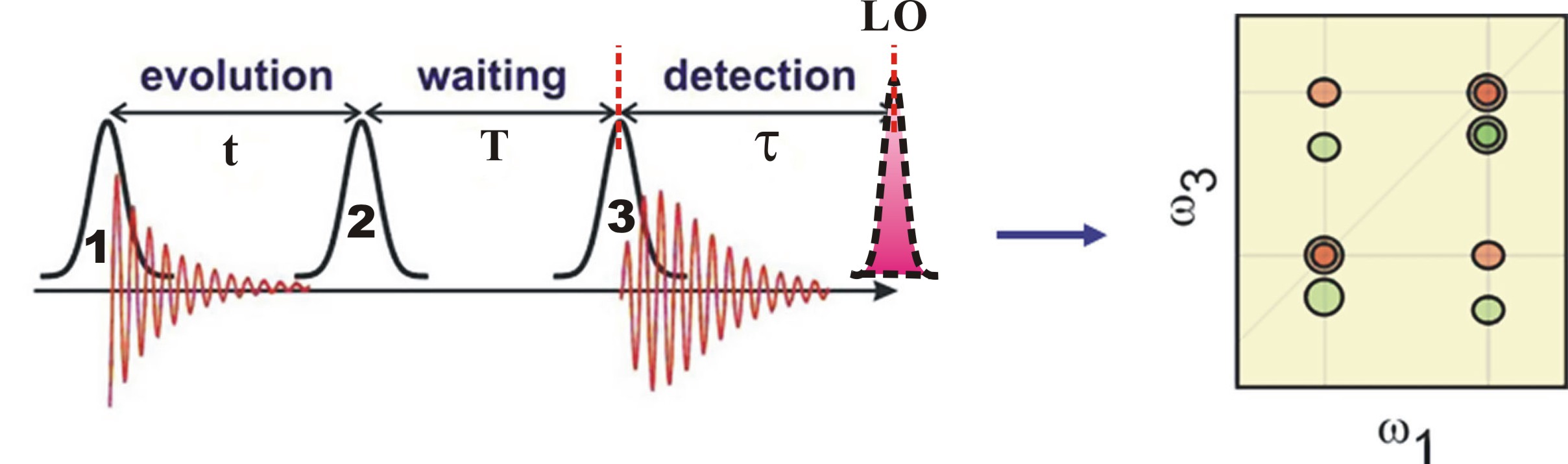
FIG. 2: Schematic showing the timing sequence of excitation pulses for heterodyne detection of 2D CS with a local oscillator (LO). The resulting 2D spectrum, generated by the third-order nonlinear optical polarization of the material system, links the dipole oscillation frequency during the initial coherence period t with that of the final rephasing period $\tau $ for each waiting time T. The shapes of peaks appearing on the diagonal provide a measure of the memory of the system, while cross-peaks provide information on electronic coupling. As a function of the waiting time T, 2D spectra measure system relaxation such as energy transfer or spectral diffusion. Thus, the 2D techniques can unfold complex and highly congested spectra by spreading them in two dimensions. 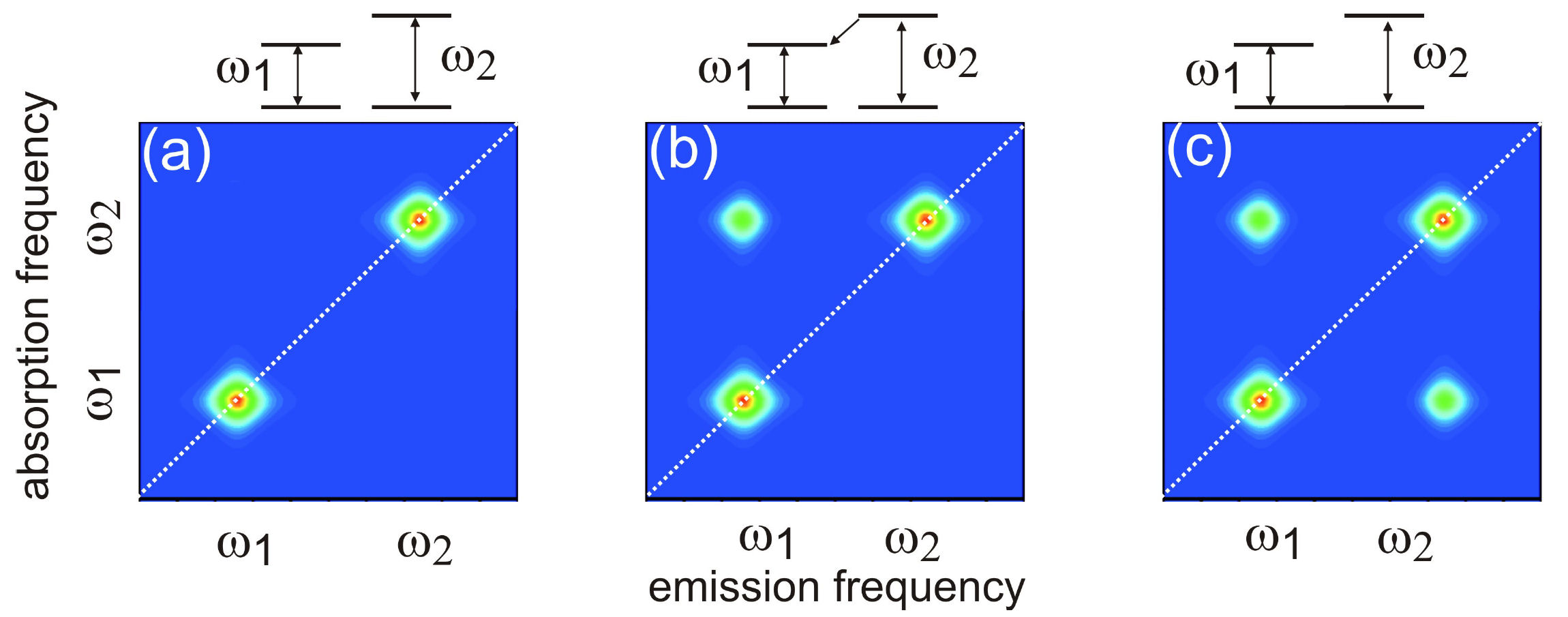
FIG. 3: Schematic diagrams illustrating the lineshapes of 2D CS as the two-level systems are mutually independent (left); coupled via excited states (center); or coupled through the ground states (right). The optical pulses-induced polarization on a molecule located at position r is given by \(P(\vec r,t)\), which can be Fourier decomposed as \(P(\vec r,t) = \sum\nolimits_{{k_s}} {{P_s}(\vec r,t)\,{e^{i\,{{\vec k}_s} \cdot \vec r}}} \), where \({\vec k_s}\), where ks are linear combinations of wavevectors of the incoming fields. Signal is produced by the radiation source iP(r, t). We can choose to study a single component \({P_s}(\vec r,t)\) in P(r, t) by detecting only the radiation in the direction \({\vec k_s}\). This specific signal detection can be achieved by interfering the radiation with a fourth pulse moving in the same direction as ks. Spatial integration over the probed volume selects out the component from \(P(\vec r,t)\). The time integration yields a signal that is proportional to the components of oscillating at the frequencies of the LO, giving by \({E_s}({\omega _\tau };\,t,T) = \frac{{2\pi l{\omega _\tau }}}{c}i{P_s}({\omega _\tau };\,t,T)\) where l denotes the sample thickness and c the light speed in vacuum. Three dimensional coherent spectroscopy can then be realized by performing multidimensional Fourier transform using \({S_{3D}}({\omega _\tau };{\omega _T},{\omega _t}) = \int {\int {{E_s}({\omega _\tau };T,t){e^{i{\omega _t}t + i{\omega _T}T}}dt\,} dT}\). 
FIG. 4: Plot of \({S_{3D}}({\omega _\tau };{\omega _T},{\omega _t}) = \int {\int {{E_s}({\omega _\tau };T,t){e^{i{\omega _t}t + i{\omega _T}T}}dt\,} dT} \), Thus the crucial step to produce a multidimensional coherent spectrum is to deduce the complex signal field \({E_s}({\omega _\tau };t,T)\). B. Spectral interferometry (SI) is a widely used technique to retrieve the phase profile of an optical field The field spectrum is defined as \({\tilde E_s}(\omega ) = \int {{E_s}(t){e^{ - i\omega t}}dt} \). By referring to Fig. 2, we can express the spectrum of signal field as a sum of \({\tilde E_s}(\omega ) = {\tilde E_{echo}}(\omega ) + {\tilde E_{LO}}(\omega ){e^{ - i\omega \tau }}\). The spectrally resolved signal detected by SI reads \({I_s}(\omega ) = {\left| {{{ \tilde E}_s}(\omega )} \right|^2} = {\left| {{{\tilde E}_{echo}}(\omega )} \right|^2} + {\left| {{{\tilde E}_{LO}}(\omega )} \right|^2} + 2\left| {{{\tilde E}_{echo}}(\omega )} \right|\left| {{{\tilde E}_{LO}}(\omega )} \right|\cos [{\phi _{echo}}(\omega ) - {\phi _{LO}}(\omega ) + \omega \tau ] \). We present in Figure 5 a measured interferogram of an echo field with a local oscillator. As we scan the arriving time of the local oscillator from the leading side (negative \(\tau \)) to the lag side (positive \(\tau \)) of the echo signal, the fringe spacing varies inversely with \(\tau \) as \(\Delta \omega = 2\pi /\tau \). At a given \(\tau \), the fringe spacing is distorted across the spectral profile, carrying the information of the relative phase \({\phi _{echo}}(\omega ) - {\phi _{LO}}(\omega )\). For a reference, the temporal separation between the two pulses varying from 0.1 ps to 1 ps, the SI fringe spacing changes from 10 THz to 1 THz. 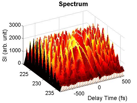
FIG. 5: Interferograms of an echo field measured as the delay time of the local oscillator used was scanned from the leading (negative delay time) to the lag side (positive delay time). C. Retrieving Phase Profile with Wavelet Transform A widely used technique to determine the spectral phase difference between two light fields is to Fourier-transform the spectral interferogram to a time domain. This procedure yields a function of three peaks. The AC component peaked at t = +τ is selected using a filter and then inversely Fourier-transformed to the frequency domain. A concatenation procedure is then used to recover the phase. However, if the spectral interferogram is modulated by a noise source with a frequency similar to the fringe spacing, the transform of this modulated signal will be close to the AC signal, and a temporal filter cannot exactly exclude such noise, resulting in the retrieved phase profile to be more or less dependent on the width of the temporal filter used. Furthermore, both the spectral resolution and nonlinear frequency sampling of a spectragraph can also result in phase measurement distortion. As shown by Y. Deng, et al, these drawbacks can be minimized by using wavelet transform (WT). Following to the work of Y. Deng, et al., we employed Morlet wavelet \(\begin{array}{c}W(x) = \frac{1}{{\sqrt {\pi a} }}{e^{2\pi i(x - b)/a}}{e^{ - {{(x - b)}^2}/{a^2 }}}\\ = \frac{1}{{\sqrt {\pi {F_b}} }}{e^{2\pi i{F_c}x}}{e^{ - {x^2}/{F_b}}}\end{array}\) , abbreviated as \(cmor{F_b} - {F_c}\), for our WT analysis of 2D CS. The wavelet transform of an SI is defined as \(\begin{array}{c}WT({I_s};a,b) = \frac{1}{{\sqrt a }}\int {{I_s}(x){W^*}(\frac{{x - b}}{a})dx} = \frac{1}{{\sqrt {\pi a} }}\int {{I_s}(x){e^{ - 2\pi i(x - b)/a}}{e^{ - {{(x - b)}^2}/{a^2}}}dx} \\ = {\left( {\frac{{2\ln 2}}{\pi }} \right)^{1/4}}\frac{1}{{\Delta f}}\int {{I_s}(f'){e^{ - 2\pi i(f' - f)/\Delta f}}{e^{ - \ln 2{{(f' - f)}^2}/{{(\Delta f)}^2}}}df'} \end{array}\) . with \(\sigma = \Delta f/\sqrt {2\pi } \), \(\tilde b = b\,\sigma = f\), and \(\tilde a = a\sigma = \Delta f/\sqrt {\ln 2} = 1.7375\Delta f\). A suitable value for the scaling factor is \(a = \sqrt {2\pi /\ln 2} = 3.0108\). At the ridge of the WT modulus, \({\tilde a_{ridge}} = a/(\sqrt {2\pi } \,\tau )\), relating to a temporal separation of \(\tau [ps] = 1.7375/{\tilde a_{ridge}}(THz)\). We use a synthesized signal \(I(x) = {e^{ - {{[(x - 0.5)/0.3]}^2}}}{e^{20\pi i{{(x - 0.5)}^3}}}\cos [20 \times 2\pi x]\) to illustrate the usage of WT for the retrieval of signal amplitude and phase profile. The synthesized data is a Gaussian profile modulating on a carrier with a frequency of 20 and a phase profile distorted by a cubic dispersion. A MatLab script is available for your testing. Figure 6 presents the WT plots of the synthesized signal as functions of the scaling factors a (Y-axis) and b (X-axis). 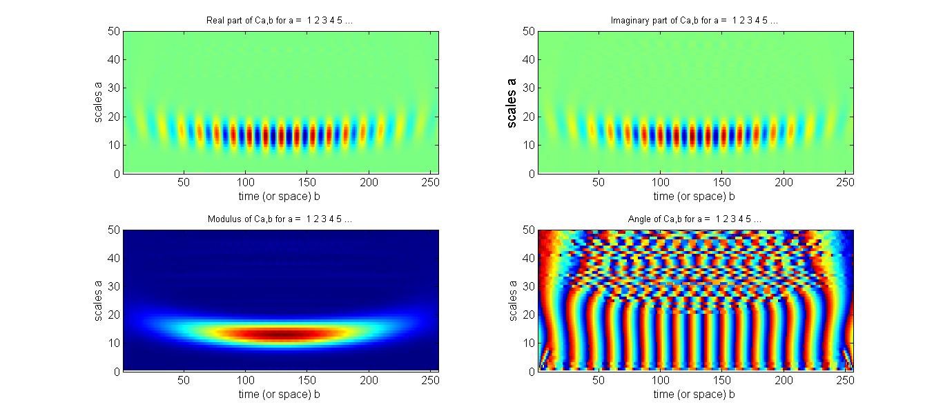
FIG. 6: WT Plots (real, imaginary, magnitude, and phase) of the synthesized signal on a functions of scaling factors a and b. As shown above, the ridge of the modulus locates between 13-14. The magnitude and phase profile of the signal can be directly read out along the ridge. Figure 7 show the comparison of the retrieved profiles (blue curve and blue symbols) with that taken from the synthesized signal (red-colored curves). The agreement is excellent as long as the scaling factor a is appropriately chosen. 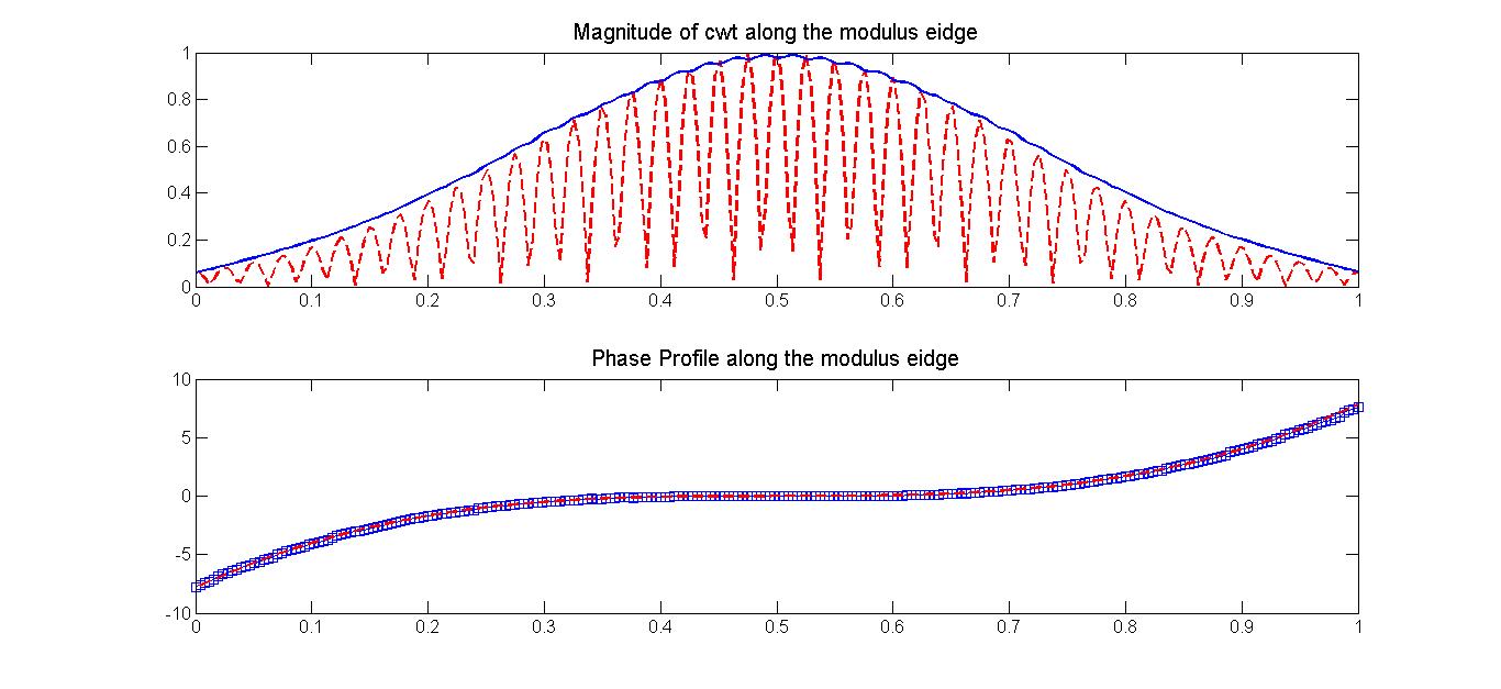
FIG. 7: Comparison of the retrieved profiles (magnitude: blue curve and phase: blue symbols) with that taken from the synthesized signal (red curves). |
2D CS of Cyanine GlassTwo-dimensional coherent spectroscopy is advantageous over other spectroscopic methods for studying quantum-confined structures because it can achieve both high spectral resolution and high temporal resolution simultaneously. To test the performance of our 2D coherent spectroscopy, we applied our apparatus to study a low bandgap cyanine glass (C3C5/BHQ10). The absorption spectrum of a 2-mm thick glass is presented in Fig. 1, which shows a broad band in the near infrared region (NIR). The excitation pulse used (the blue dashed curve) has a bandwidth much narrower than the NIR absorption spectrum. Therefore only a fraction of the cyanine molecules embedded in the glass matrix was excited. The echo signal emitted from the excited molecules has a spectral profile (the red solid curve) similar to that of the excitation pulses and the local oscillator. The Matlab script used to process our 2D CS data is also available here with 2D CS data set and LO spectrum. 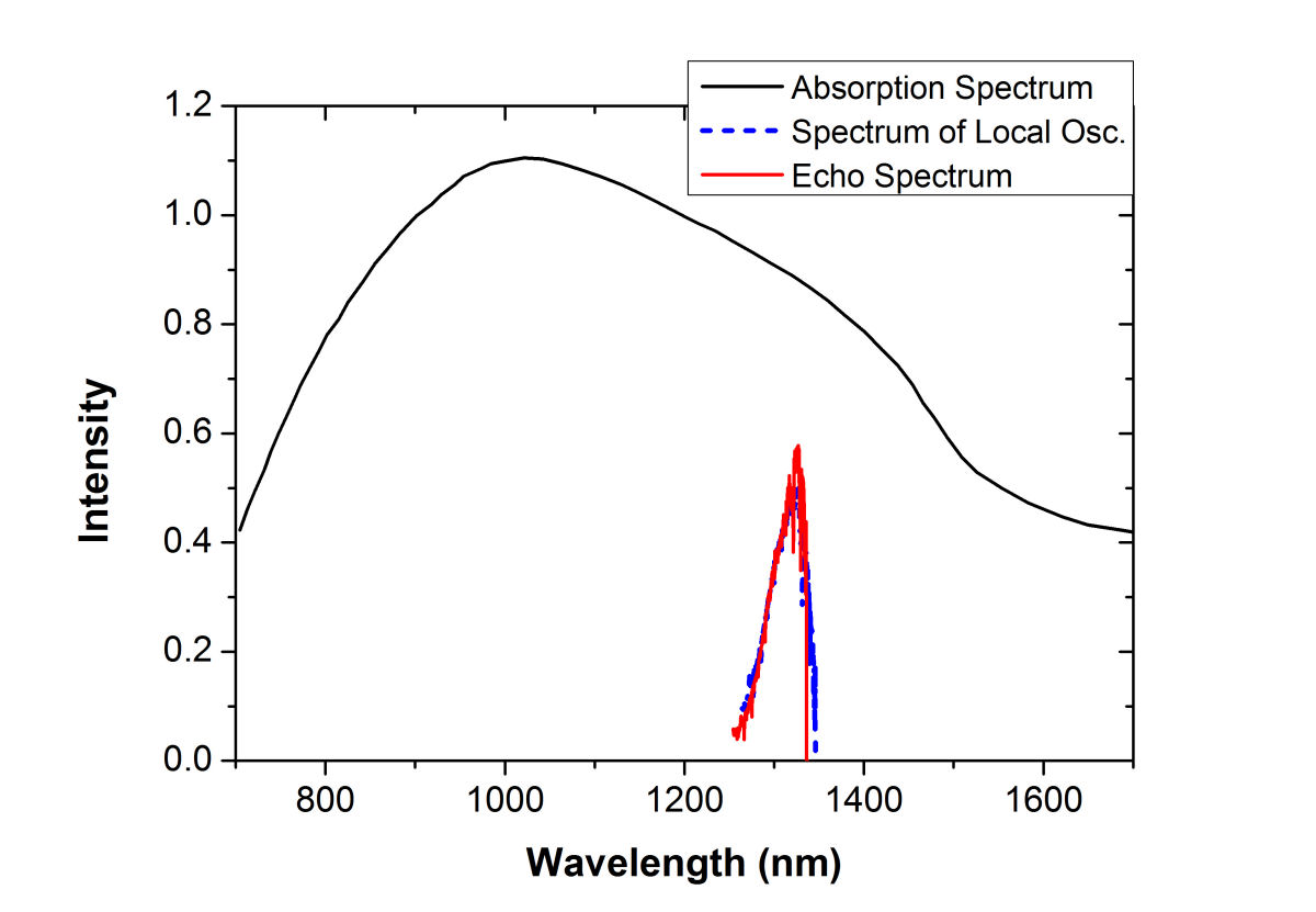
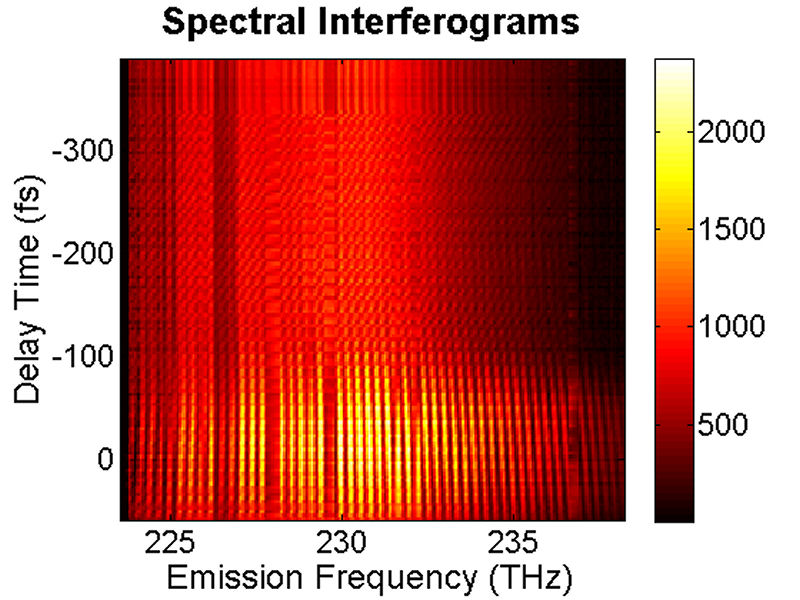
FIG. 1: Absorption spectrum (black curve) of a 2-mm thick cyanine glass plate and the spectra of the local oscillator (blue dashed curve) and photon echo signal (red solid curve) emitted from the glass plate. By blocking individual excitation pulses, the photon echo signal drops to the background level since the photon echo signal depends on a three-pulse excitation. By scanning the delay time t of the pulse 1 (relative to the pulse 2) while keeping the delay time T of the third pulse at 0 fs, the spectral interferograms of the echo signal with the LO can be acquired and are presented in Fig. 2(a).
(a)
 ...
(b)
...
(b)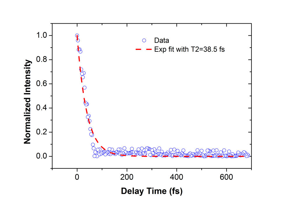
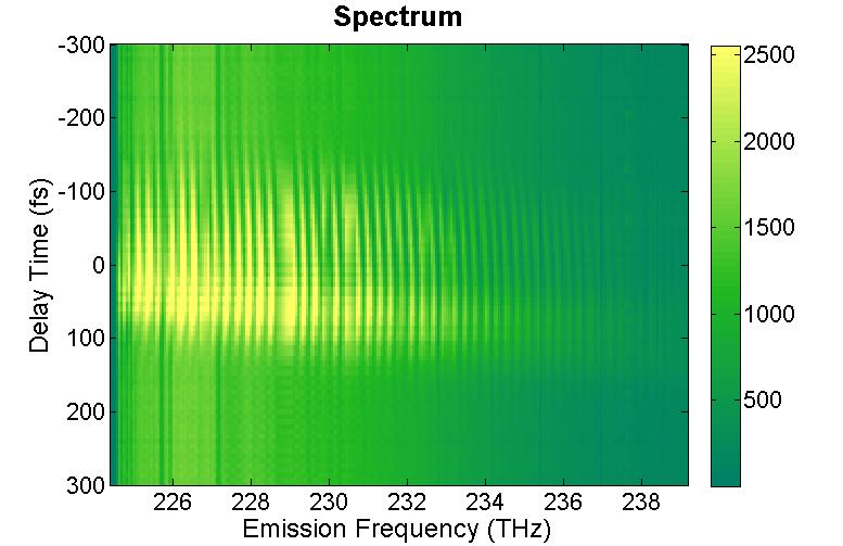
FIG. 2: (a) Spectral interferograms of echo signal field emitted from a 2-mm thick cyanine glass plate acquired by scanning the coherent delay time from -350 to +50 fs. (b) The integrated spectral intensities (open circles) plotted as a function of the coherent delay time and the exponential fit (red dashed curve). We can fit the integrated spectral intensities to an exponentially decaying curve and gives a dephasing time of 39 fs. This measured dephasing time suggests a homogeneous linewidth \(\Delta {E_{FWHM}} = 34\;meV = 276\;c{m^{ - 1}}\) using \(\Delta {E_{FWHM}} = 1316.4[meV.fs]/t[fs]\). By scanning the delay time T of the third pulse while keeping the coherent delay time at t=0, the resulting spectral interferograms are shown in Fig. 3. The energy relaxation rate of the cyanine molecules embedded in a glass matrix can be deduced from the decay curve with respect to the delay time T, yielding an energy relaxation time of 54 fs. The fast energy relaxation rate is caused by the strong coupling of the optical excitation with phonons of the glass matrix.
(a)
 ...
(b)
...
(b) 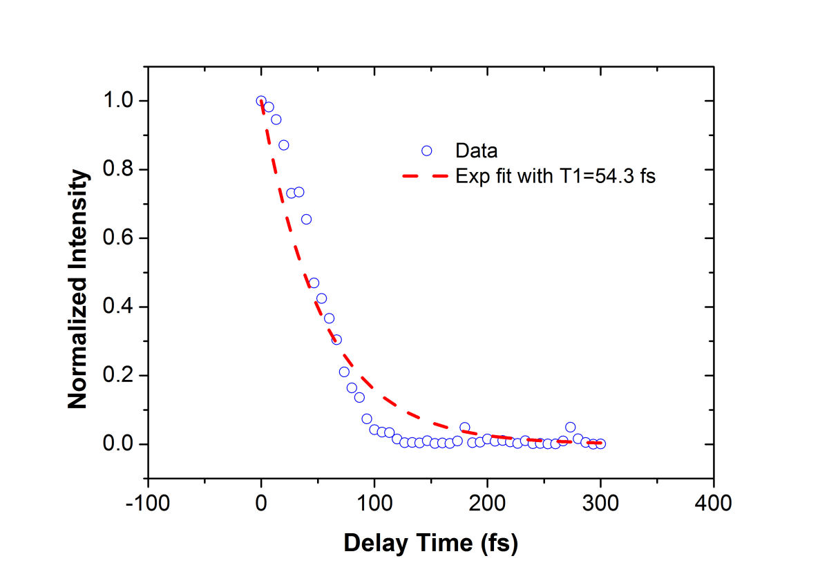
FIG. 3: (a) Spectral interferograms of echo signal field acquired by scanning T from -300 to +300 fs while keeping t=0 fs. (b) The integrated spectral intensities (open circles) plotted as a function of T and the exponential fit (red dashed curve). In order to get a flat phase across the proper frequency range, the time delay between the echo signal and LO field must be chosen properly in processing the data. As shown in Fig. 4, our 2D CS apparatus has a long-term stability to produce clean spectral interferograms as \({\tau _W}\) is scanned from -200 fs to 900 fs. Typically, we choose \({\tau _W}\) to be between 700 fs and 1 ps. 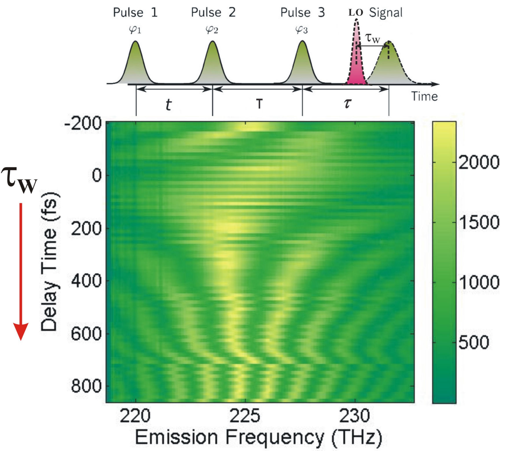
FIG. 4: Spectral interferograms of an echo field as the delay time of the LO used is varied from the leading side (-200 fs) to the lag side (+800 fs). The retrieved magnitude of \({\vec E_{echo}}({\omega _\tau };T,t)\) as a function of t is presented in Fig. 5. 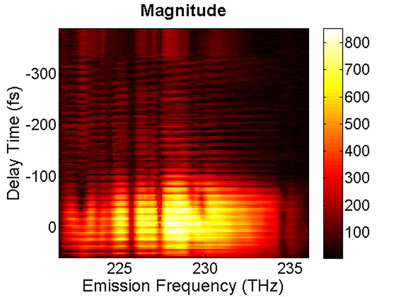
FIG. 5: The magnitude of \({\vec E_{echo}}({\omega _\tau };T,t)\) is shown on the range of t from -400 to 50 fs with T fixed at 0 fs. By Fourier transforming \({\vec E_{echo}}({\omega _\tau };T,t)\) over the coherence time interval t, we can produce a 2D CS plot. The magnitude of \({S_{2D}}({\omega _\tau };T,{\kern 1pt} {\omega _t})\) is shown in Fig. 6. Here \({\omega _\tau }\) is called as “emission frequency”, whereas \({\omega _t}\) termed as “excitation frequency”. 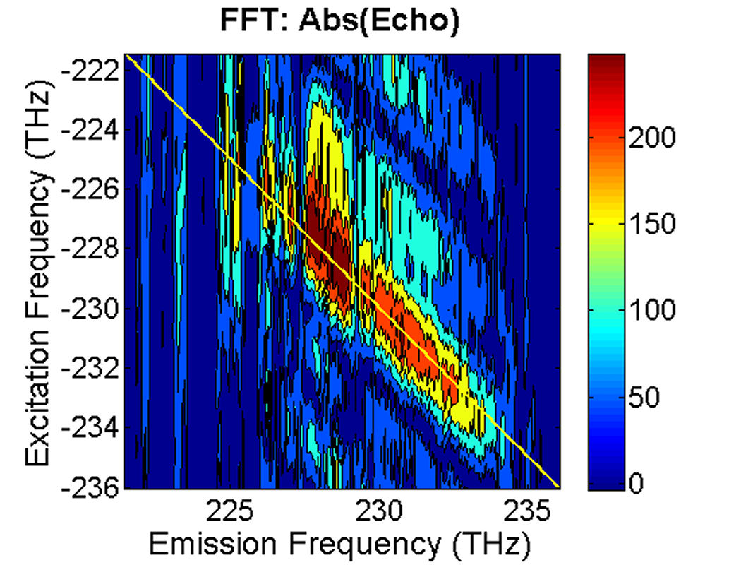 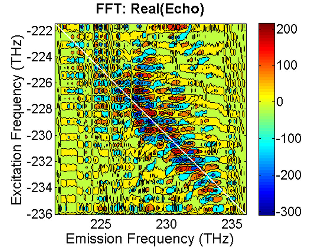
FIG. 6: Plots of the magnitude and real part of \({S_{2D}}({\omega _\tau };T,{\kern 1pt} {\omega _t})\) at T=0 fs. The echo field spectrum is similar to that of the excitation pulses (see the red solid and the blue dashed line of Fig. 1), giving a crowd of diagonal peaks on the 2D CS plot. They are most likely contributed by cyanine molecules embedded in different environments. Although this inhomogeneous broadening renders the absorption spectrum of the glass sample to an extremely broad and featureless profile, the rephasing process invoked in the 2D CS technique recovers the linewidth of different molecules at their homogeneous dephasing limit and hence was resovable in the 2D CS plot. Weak off-diagonal peaks can also be observed. But due to the complicated diagonal peak structure, the cross peaks can not be confidently defined. |
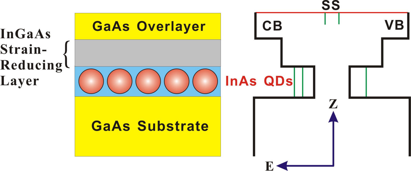
2D CS of InAs quantum dots beneath a strain-reducing layerSemiconductor quantum dots (QDs) are promising candidates for a number of optoelectronic applications. However, photoluminescence (PL) of InAs quantum dots (QDs) strongly depends on their distances to the device surface. Therefore, to improve the absorption/emission efficiency of photons, it is necessary to reduce the surface loss of optically excitted carriers. For example, we can employ an overgrown strain-reducing layer on InAs QDs to tailor the carrier confinement and the absorption band of the optically active medium. The schematic of the devices under study and their band structure are shown in Fig. 1. The PL spectra of the devices with different types of strain-reducing layers (S3355: InGaAs (blue solid line), S3357: InGaAsSb) (red dashed curve) are presented on the right hand side of the figure. The result shows that the electronic energy structure of InAs QDs can be modified by a carefully designed strain-reducing layer.
(a)
 ...
(b)
...
(b)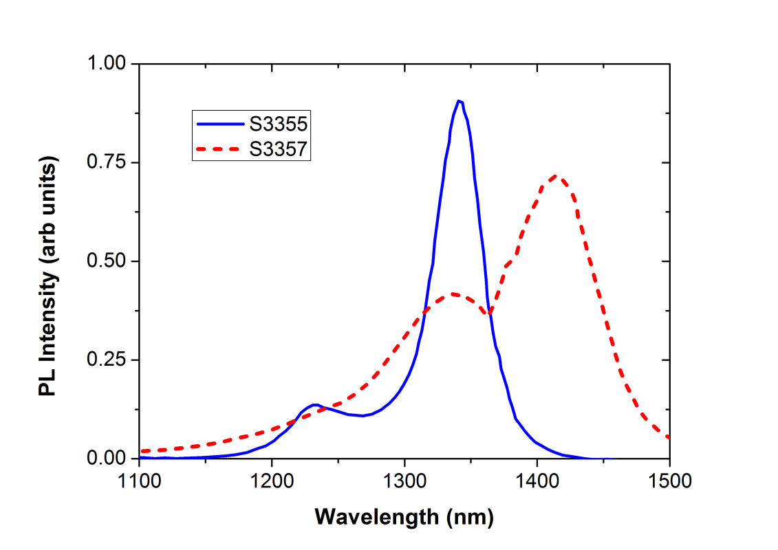
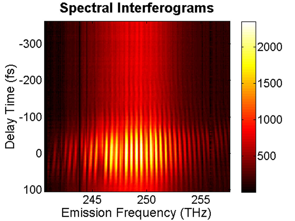
FIG. 1: (a) Schematic of the device structure S3355 and (b) the corresponding PL spectra measured at T=300 K. S3355: with a strain-reducing layer of InGaAs (blue solid line), S3357: with a strain-reducing layer of InGaAsSb (red dashed curve). To decipher the coherent dynamics of optically excited carriers in the quantum confined structures, we employed 2D CS technique to study the coupling effects in InAs QDs and between InAs QDs and the strain-reducing layer. The device was excited by four ultrashort laser pulses with a spectrum covering from 1164 nm (258 THz) to 1246 nm (240 THz), in a boxcar phase-matching geometry. The time delay t between pulse 1 and 2 was adjusted and the echo signal generated was mixed with a local oscillator. The resulting time-delayed spectral inteferograms recorded at T=0 fs with a NIR CCD is shown on the left side of Fig. 2. The delay time t (dephasing) dependence of the integrated spectral intensity curves measured at three different waiting times T are presented in Fig. 2(b). As shown, the link of the dipole oscillation activity during the initial dephasing period t with that of the final rephasing period
(a)
 ...
(b)
...
(b)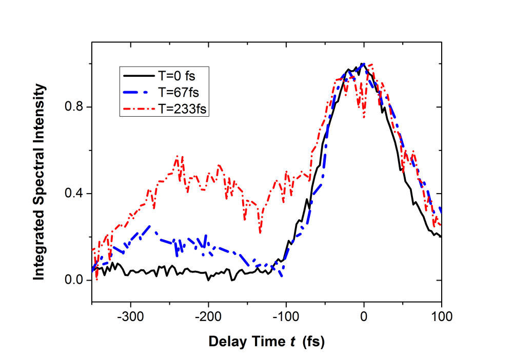
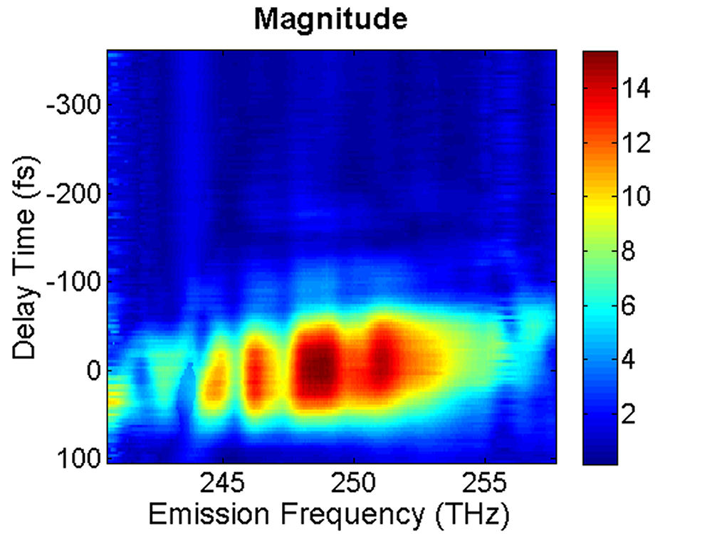
FIG. 2: (a) Spectral interferograms of echo light field emitted (with a central wavelength 1200 nm) from InAs QDs self assembled in the structure of Fig. 1. (b) The t (dephasing) dependence of the integrated spectral intensity curves measured at three different T (waiting time). We extracted the modulus and phase of the echo field from the spectral interferograms. The retrieved amplitudes of the echo field acquired at T=0 fs and T=100 fs are presented in Fig. 3.
(a)
 ...
(b)
...
(b)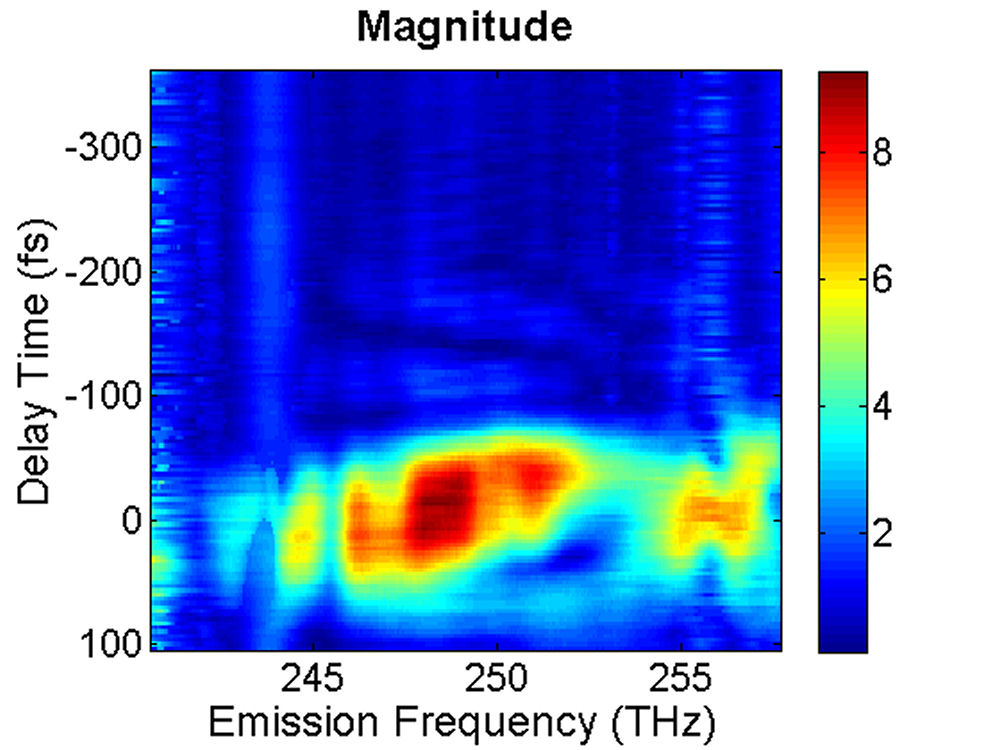
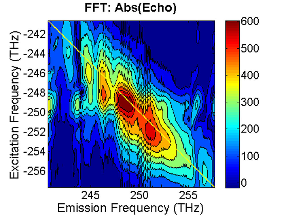
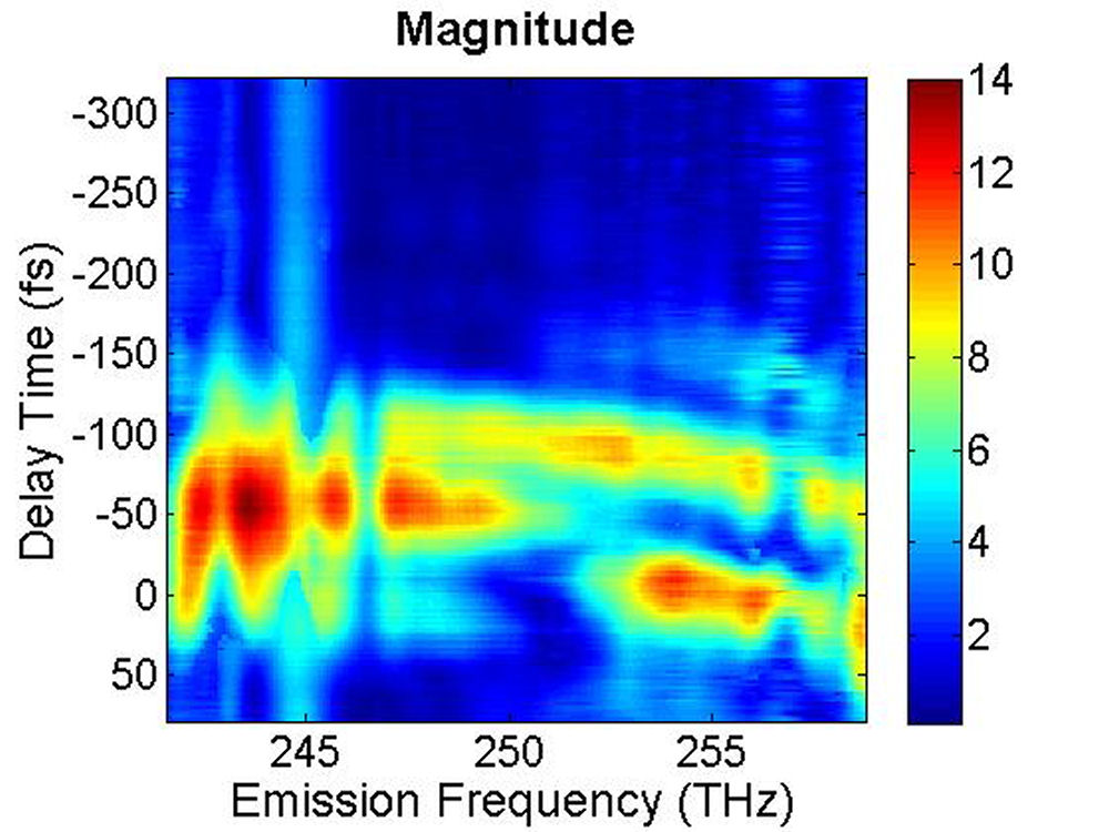
FIG. 3: Time-delayed echo field amplitude at (a) T=0 fs and (b) T=100 fs retrieved with the method illustrated in Sec. 1. We Fourier transformed the echo field over the delay time t to form the 2D plot of the echo field. The resulting magnitudes of \({S_{2D}}({\omega _\tau };T,{\kern 1pt} {\omega _t})\) at (a) T=0 fs, (b) 67 fs, (c) 100 fs, and (d) 233 fs are shown in Fig. 4. The appearance of the cross peaks at one side of the diagonal line indicates that the excited states of InAs QDs are coupled. Although the first PL peak from the exciton 1e->0h of the device is broad and ranges from 1160 nm to 1260 nm, two major peaks at (249, -249) and (251,-252) THz can be clearly resolved due to the rephasing process of 2D CS. The main peak at (249, -249) persists up to T=233 fs without changes its position and shape. However, the peak at (251, -252) first switches to (251, -249) at T=67 fs due to a ultrafast cross coupling with the main peak at (249, -249). The coupling quickly damps out, causing the cross peak to return to (251, -252) at T=233 fs.
(a)
 ...
(b)
...
(b)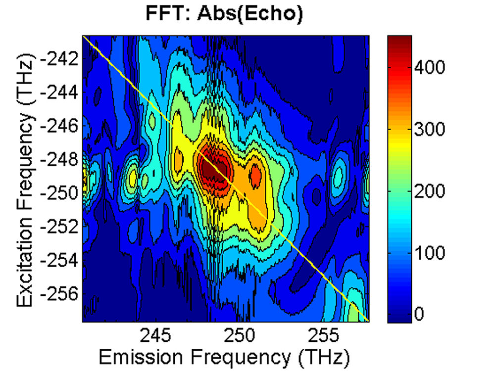
(c) 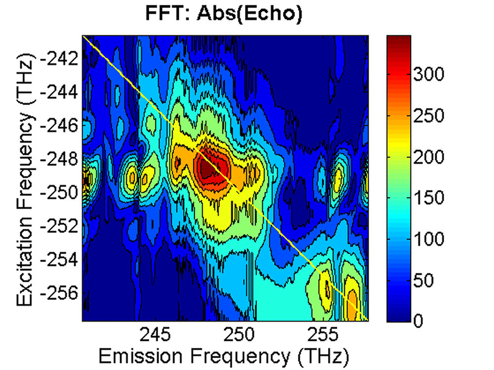 ...
(d)
...
(d)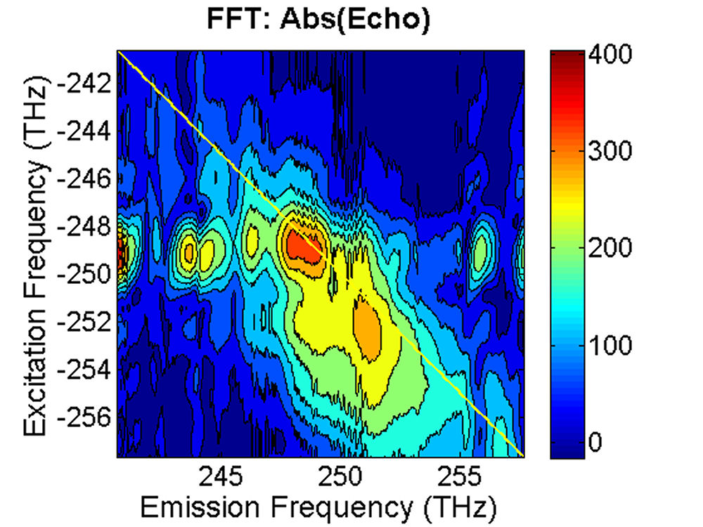
FIG. 4: Plots of the magnitude of \({S_{2D}}({\omega _\tau };T,{\kern 1pt} {\omega _t})\) at (a)T=0 fs, (b) 67 fs, (c) 100 fs and (d) 233 fs. The frequency difference between two neighboring diagonal peaks is about 2-3 THz, corresponding to 67-100 \(c{m^{ - 1}}\) splitting. The splitting is about a factor of 2.5 lower than the calculated value of TO and LO modes in an InAs QD. InAs possesses a nonvanishing piezoelectric effect (\({\left. {\partial Q/\partial E} \right|_{{Q_0}}} \ne 0\)), thus the ultrashort optical pulses \(E\) used in 2D CS can generate a lattice distortion \(Q\) in accompany with the exciton generation. The resulting exciton-acoustic phonon coupling can contribute to the 2D CS signal via a modulation on the third-order nonlinear optical susceptibility \(\Delta {\chi ^{(3)}} = {\left. {\partial {\chi ^{(3)}}/\partial Q} \right|_{{Q_0}}} \cdot {\left. {\partial Q/\partial E} \right|_{{Q_0}}}\). Thus it is possible that the observed ultrafast switching of the cross peak reflects an appearance of exciton-acoustic phonon coupling in InAs QDs. The response time reflects the built up dynamics of phonon amplitude, which was found to last up to 230 fs. Such coherent coupling phenomenon can only be observed with 2D CS because the technique offers both high spectral resolution and high temporal resolution simultaneously. More... |
2D CS of Lead Sulfide Quantum Dots in SolutionA. PbS Quantum Dots (\({\lambda _{em}}\)=1200 nm) Suspended in Toluene PbS QDs in pure toluene form a large population of absorbers. We are interested to probe the sub-100 femtosecond dynamics of these free absorbers with 2D CS. The PbS QD samples used for this study have a well-defined size distribution and yield a very clean 1s exciton absorption peak (the blue curve in Fig. 1) at 1150 nm. Unlike GaAs, which yields two peaks for heavy-hole (HH) and light-hole LH), PbS QDs exhibit much more inhomogenously-broadened spectra. Our excitation pulse has a bandwidth narrower than the 1s absorption peak. Therefore only a fraction of the 1s absorbance band near the edge was excited. The dephasing rate of PbS QD between several different excited states had been measured and calculated previously to be about sub-10 fs at room temperature. Single-dot studies at 300K had yielded linewidths of 100 meV, also indicating sub 100 fs dephasing in PbS QDs. The ultrafast dephasing in PbS could be attributed to coupling with acoustic phonons. Overlapping electron and hole wavefunctions due to strong confinement in these lead-chalcogenide QDs can be significantly influenced by coupling to phonons at four L valleys and at X-points. Particularly, the X-points, which were known to have a large phonon density of states. Our excitation pulse width is broad enough in spectrum and can excite multiple phonon modes simultaneously. Thus, the dephasing would have contributions from several acoustic and optical phonon branches. 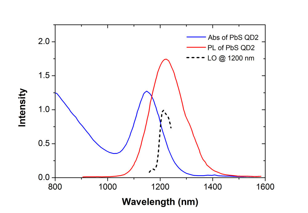
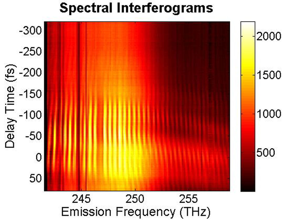
FIG. 1: Absorption (blue solid curve) and fluorescent spectra (red solid curve) of PbS quantum dots in toluene. The spectra of the local oscillator (black dashed curve) and the photon echo signal (pink) are also included for comparison. Due to the limitation of our NIR spectragraph, wavelength of LO higher than 1250 nm was not recorded. We employed 2D CS technique to investigate these PbS QD absorbers in Toluene. The sample under study was excited by four ultrashort laser pulses with a spectrum covering from 1164 nm (258 THz) to 1246 nm (240 THz) in a boxcar phase-matching geometry. The time delay between pulse 1 and 2 was adjusted and the echo signal generated was mixed with a local oscillator (see the dashed curve in Fig. 1). The resulting time-delayed spectral inteferograms recorded at T=0 fs with a NIR CCD are shown in Fig. 2(a). The dephasing time dependent curves of the integrated spectral intensity measured at three different waiting times (T=0, 67, and 100 fs) are presented in Fig. 2(b). In ccontrast to the case of InAs underneath the strain-reducing layer, the link of the dipole oscillation activity during the initial dephasing period with that of the final rephasing period decreases as the waiting time increases.
(a)
 ...
(b)
...
(b)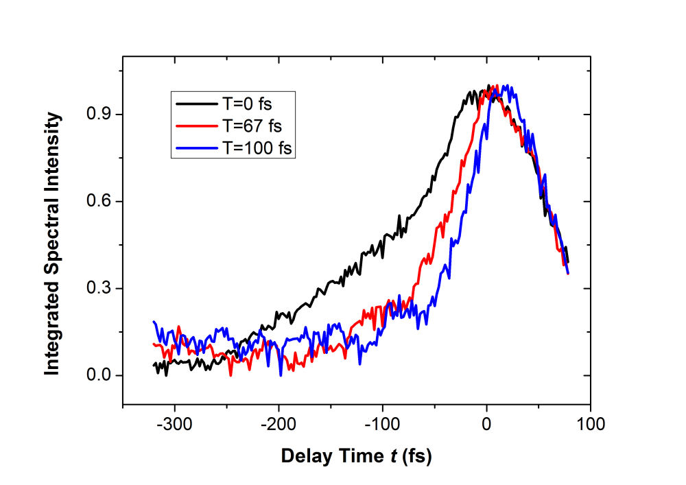
FIG. 2: (a) Spectral interferograms of echo signal field emitted from the PbS quantum dots in toluene acquired by scanning the coherent delay time from 75 fs (larer pulse 1) to -325 fs (earlier pulse 1). (b) The dephasing time t dependent curves of the integrated spectral intensity measured at three different waiting times (T=0 fs. 67 fs, and 100 fs). The magnitude of \({\vec E_{echo}}({\omega _\tau };T,t)\) as a function of t is presented in Fig. 3. For optical excitation at the long-wavelength tail of the 1s exciton absorption peak, the dynamic emission process starts at t=-100 fs with spectrum first centered at 252 THz. By reducing the coherent evolution time, the dynamic spectrum shifts to 244 THz and then back to 254 THz. The dynamic emission processes change significantly at T=100 fs as shown in Fig. 2(b).
(a)
 ...
(b)
...
(b)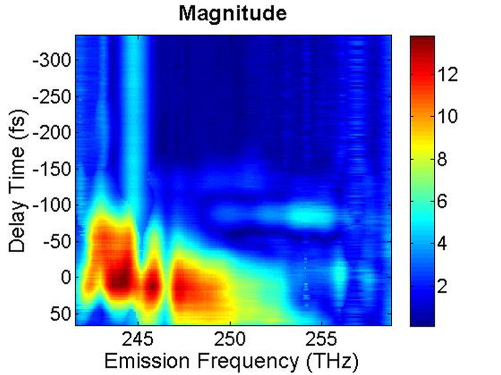
FIG. 3: The magnitude of \({\vec E_{echo}}({\omega _\tau };T,t)\) emitted from the quantum dots is shown on the range of t from -350 to 100 fs with T fixed at (a) 0 fs, and (b) 100 fs. The magnitude of the 2D CS is shown in Fig. 4. Several bands are visible along the diagonal of the 2D CS plot. Distinguishing these states is only possible with techniques that allow both high spectral and temporal resolution. The appearance of multiple peaks along the diagonal, whose peak amplitudes decay with T, is consistent with recent calculations by Zunger that suggest intervalley splitting in small PbSe QDs on the order of 20 meV. The major finding is that the significant echo emission activity occurs at 253 THz (1185 nm). The blue-shifted emission disappears completely at T=100 fs. The complex 2D CS lineshape of PbS QDs is due to the inhomogeneous broadening, which could originate from the size and shape distribution of PbS quantum dots. Furthermore, some intrinsic inhomogeneous broadening, which can result from fluctuations in the atomic structure within each dot, can couple to the homogeneous broadening.
(a)
 ...
(b)
...
(b)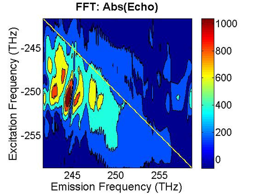
FIG. 4: The magnitude of \({S_{2D}}({\omega _\tau };T,{\kern 1pt} {\omega _t})\) at (a)T=0 fs and (b) 100 fs. B. PbS Quantum Dots with \({\lambda _{em}}\)=1400 nm We also studied a sample of PbS QDs with slightly larger diameter. The sample gives an absorption spectrum with the 1s exciton absorption peak at 1350 nm (see Fig. 5). We first excite the sample at the high energy side (blue curve) of the 1s exciton absorption peak. 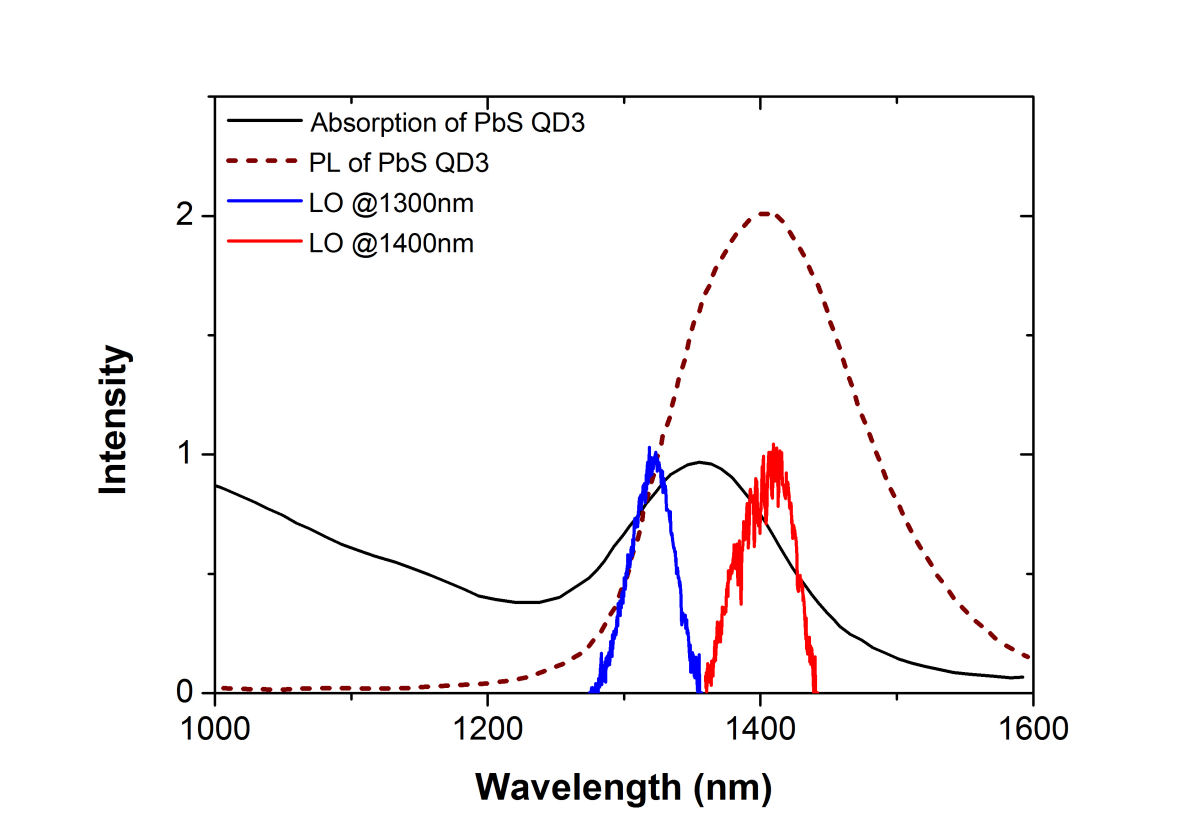
FIG. 5: Absorption (black solid curve) and fluorescent spectra (black dashed curve) of PbS quantum dots in toluene. The spectra of the two local oscillators used are shown in blue and red. The spectral interferograms of the echo signal at room temperature are presented in Fig. 6(a) and (b).
(a)
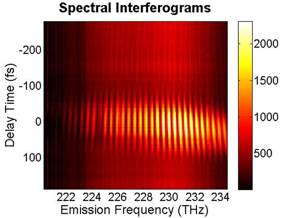 ...
(b)
...
(b) 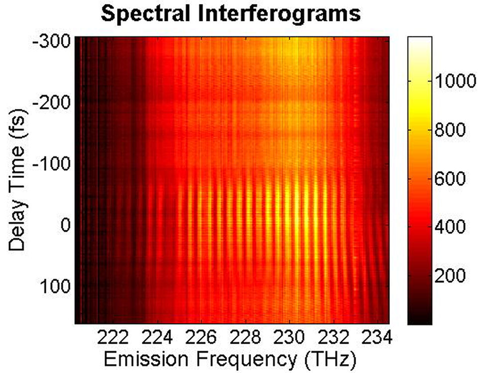
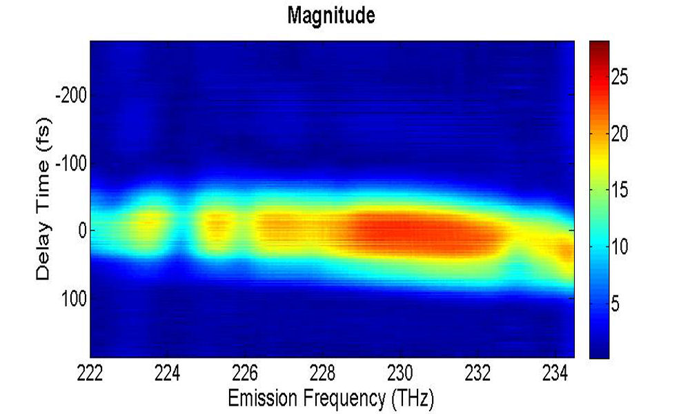
FIG. 6: Spectral interferograms of echo signal field emitted from the PbS quantum dots are shown on the range of t from -300 to 150 fs with T fixed at (a) T=0 fs, (b) T=113 fs. We deduced the echo field \({\vec E_{echo}}({\omega _\tau };T,t)\) from the spectral interferograms. Fig. 7(a) shows the magnitude of the echo field at T=0 fs. By Fourier transforming \({\vec E_{echo}}({\omega _\tau };T,t)\) over t, we can obtain the 2D CS plot as shown in Fig. 7(b). This 2D CS plot reveals a major diagonal peak at (230, -230) THz with other features at (223, -227), (225, -227), and (233, -231) THz. The energy difference between two neighboring features is about 3-5 THz in emission frequency, corresponding to 12-24 meV splitting. The appearance of multiple peaks along the diagonal is consistent with recent calculations by Zunger that suggest intervalley splitting in small PbSe QDs on the order of 20 meV for 3-nm dots.
(a)
 ...
(b)
...
(b)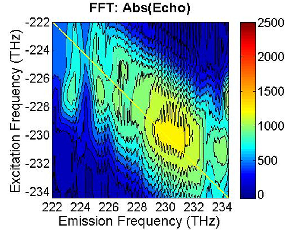
FIG. 7: (a) The magnitude of \({\vec E_{echo}}({\omega _\tau };T,t)\) emitted from the quantum dots with T=0 fs. (b) The magnitude of \({S_{2D}}({\omega _\tau };T,{\kern 1pt} {\omega _t})\) at T=0 fs As the waiting time increases, these 2D CS features appear to decay with similar relaxation rates, suggesting the dephasing process of these peaks is influenced by the same exciton-phonon coupling mechanism.
(a)
 (b)
(b)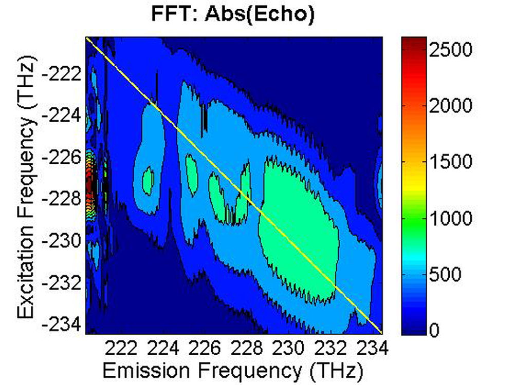 (c)
(c)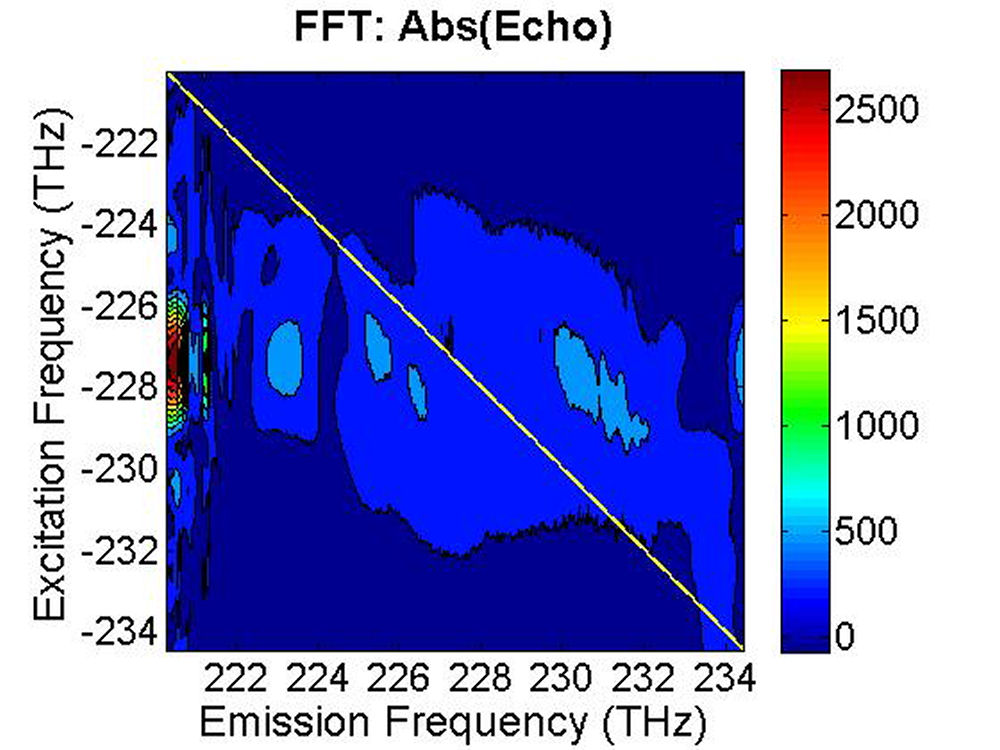
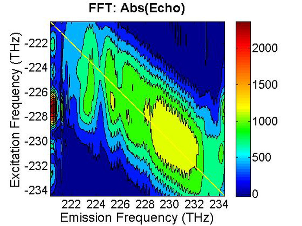
FIG. 8: The magnitude of \({S_{2D}}({\omega _\tau };T,{\kern 1pt} {\omega _t})\) recorded at (a) T=33 fs, (b) T=66 fs, and (c) T=133 fs. |